Section I
Artificial Neural Networks, Part I
Week 2 • Foundations of Training
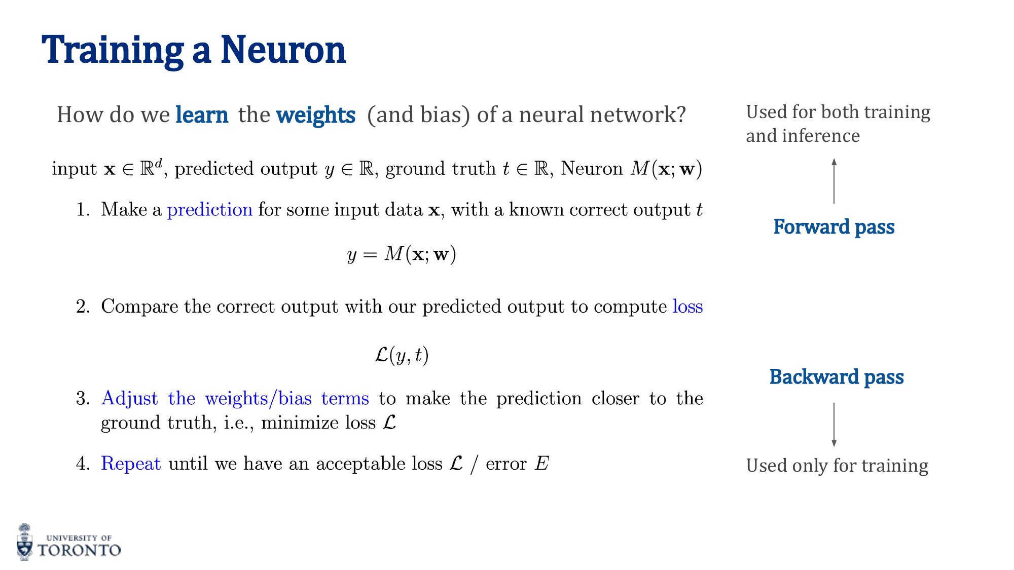
Training a neural network is an iterative optimization process. At its core, the network makes a prediction (forward pass), measures how wrong it was (loss computation), calculates how each weight contributed to the error (backward pass), and then adjusts the weights to reduce that error (weight update). This cycle repeats until the network converges to a satisfactory level of performance.
The Training Loop
Every training iteration follows four steps:
- Forward Pass: Input data flows through the network layer by layer, producing a prediction
y_hat. - Loss Computation: A loss function measures the discrepancy between the prediction
y_hatand the true targety. - Backward Pass (Backpropagation): Gradients of the loss with respect to every weight are computed using the chain rule.
- Weight Update: Weights are adjusted in the direction that reduces the loss, scaled by the learning rate.
Loss Functions
The choice of loss function depends on the task type:
Mean Squared Error (MSE) — Regression
MSE penalizes large errors quadratically. Suitable for continuous outputs (e.g., predicting housing prices, temperature).
Cross-Entropy Loss — Classification
Cross-entropy measures the divergence between the predicted probability distribution and the true distribution. It is the standard loss for multi-class classification problems.
Binary Cross-Entropy — Two-Class Problems
Used for binary classification (e.g., spam vs not spam, real vs fake). The output is a single sigmoid probability.
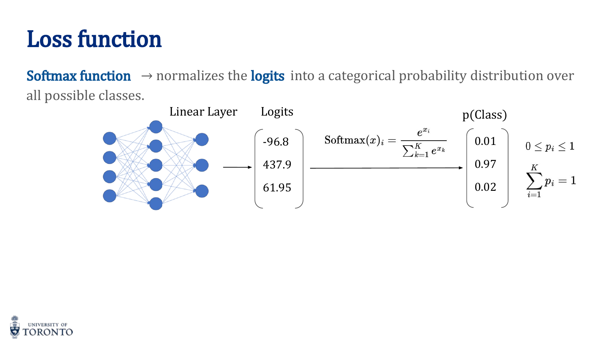
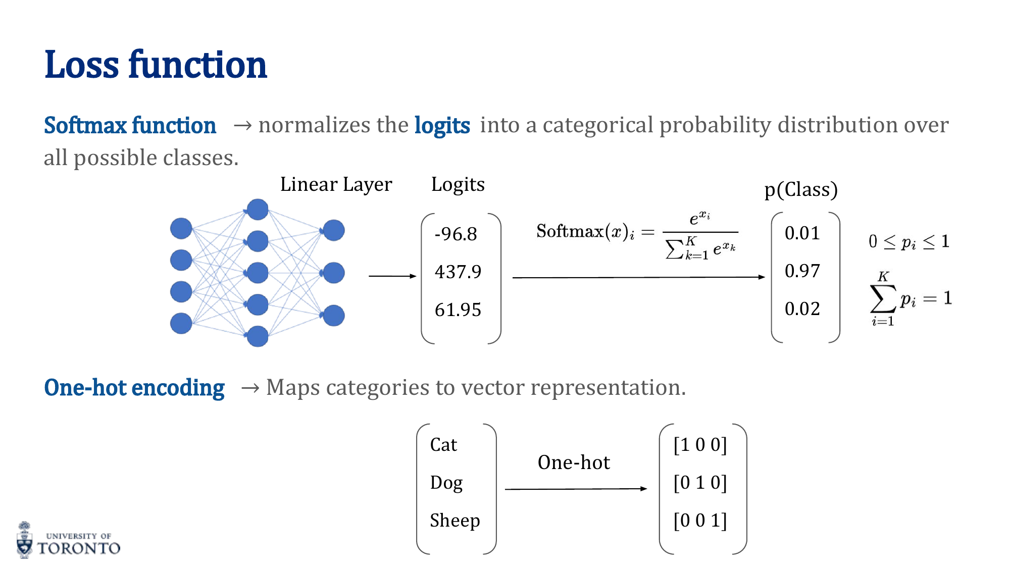
Softmax Function
The softmax function converts raw logits (unnormalized scores) into a valid probability distribution where all values sum to 1:
Each output is in the range (0, 1), and the outputs are mutually exclusive. Softmax is applied as the final layer in multi-class classification networks.
One-Hot Encoding
For categorical labels, one-hot encoding converts each class into a binary vector with a single 1:
Cat  = [1, 0, 0]
Dog  = [0, 1, 0]
Bird = [0, 0, 1]
This enables cross-entropy loss to compare the predicted probability vector against the true label vector.
Gradient Descent
Gradient descent is the optimization algorithm that adjusts weights to minimize the loss function:
Where γ (gamma) is the learning rate, controlling the step size. The gradient ∂E/∂w indicates the direction of steepest ascent, so we move in the negative direction.
Backpropagation
Backpropagation computes gradients efficiently using the chain rule of calculus. For a composition of functions f(g(h(x))), the derivative is:
Starting from the loss, gradients flow backward through each layer, allowing every weight in the network to be updated proportionally to its contribution to the error.
Activation Functions
Activation functions introduce non-linearity, allowing networks to learn complex patterns:
| Function | Formula | Range | Notes |
|---|---|---|---|
| Sigmoid | σ(x) = 1 / (1 + e^(-x)) | (0, 1) | Output interpretable as probability; suffers vanishing gradients |
| Tanh | tanh(x) = (e^x - e^(-x)) / (e^x + e^(-x)) | (-1, 1) | Zero-centered; still suffers vanishing gradients |
| ReLU | f(x) = max(0, x) | [0, ∞) | Most popular; solves vanishing gradient; can have "dead neurons" |
| Leaky ReLU | f(x) = max(0.01x, x) | (-∞, ∞) | Small slope for negatives; prevents dead neurons |
Key Insight
Vanishing Gradient Problem: Sigmoid and Tanh squash inputs into small ranges. When many layers are stacked, gradients shrink exponentially during backpropagation (multiplying many small numbers). ReLU solves this because its gradient is either 0 or 1, allowing gradients to flow unchanged through active neurons.
# PyTorch: Simple Neural Network
import torch
import torch.nn as nn

model = nn.Sequential(
    nn.Linear(784, 128),
    nn.ReLU(),
    nn.Linear(128, 64),
    nn.ReLU(),
    nn.Linear(64, 10),
    nn.Softmax(dim=1)
)

criterion = nn.CrossEntropyLoss()
optimizer = torch.optim.SGD(model.parameters(), lr=0.01)

# Training step
output = model(x)          # Forward pass
loss = criterion(output, y) # Loss
loss.backward()             # Backward pass
optimizer.step()            # Weight update
optimizer.zero_grad()       # Clear gradients
Section II
Artificial Neural Networks, Part II
Week 3 • Hyperparameters, Optimization & Regularization
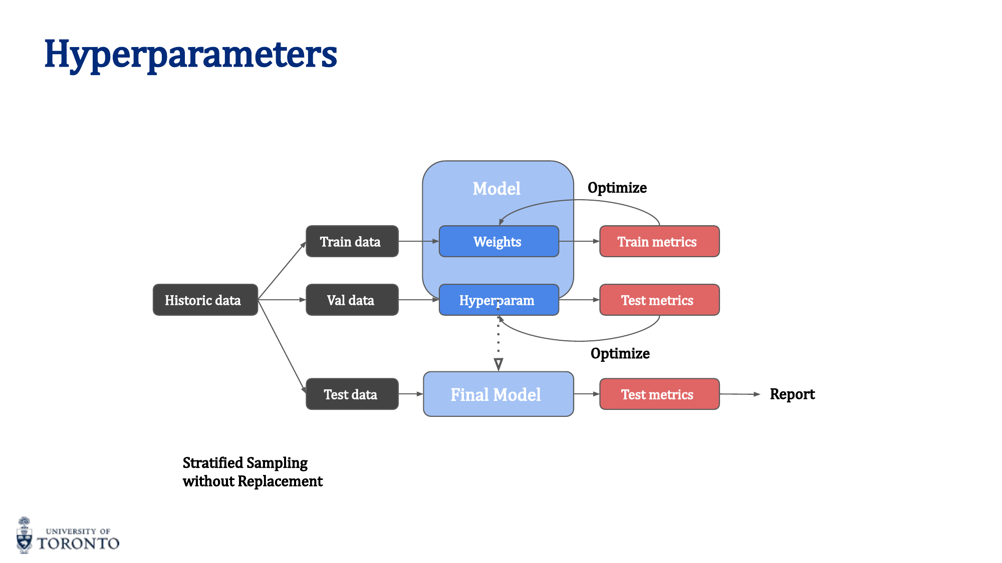
While model parameters (weights and biases) are learned during training, hyperparameters are set before training begins and govern the learning process itself. Choosing the right hyperparameters is critical: they determine the architecture, the optimization dynamics, and ultimately whether the network generalizes well to unseen data.
Hyperparameters vs Parameters
Parameters (weights, biases) are optimized during the inner training loop via gradient descent. Hyperparameters are set in the outer loop and include:
- Batch size
- Number of layers and layer sizes
- Activation function choice
- Learning rate and schedule
- Regularization strength
- Optimizer choice
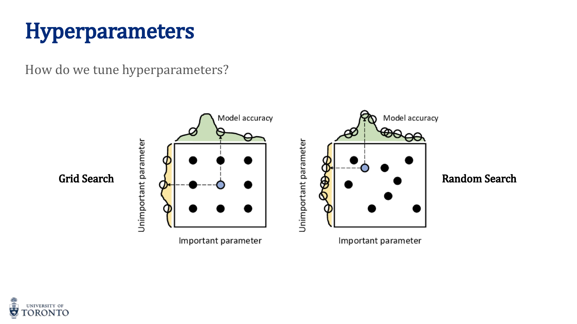
Hyperparameter Search
Two main strategies for finding good hyperparameters:
- Grid Search: Exhaustively tries all combinations of a predefined set of values. Exponential cost. Can miss good values between grid points.
- Random Search: Samples hyperparameters randomly from distributions. Generally more efficient because it explores more unique values per hyperparameter. Recommended in practice.
Optimizers
Stochastic Gradient Descent (SGD)
Updates weights using a single training sample (or mini-batch) at a time. Noisier than batch gradient descent but computationally cheaper and can escape local minima.
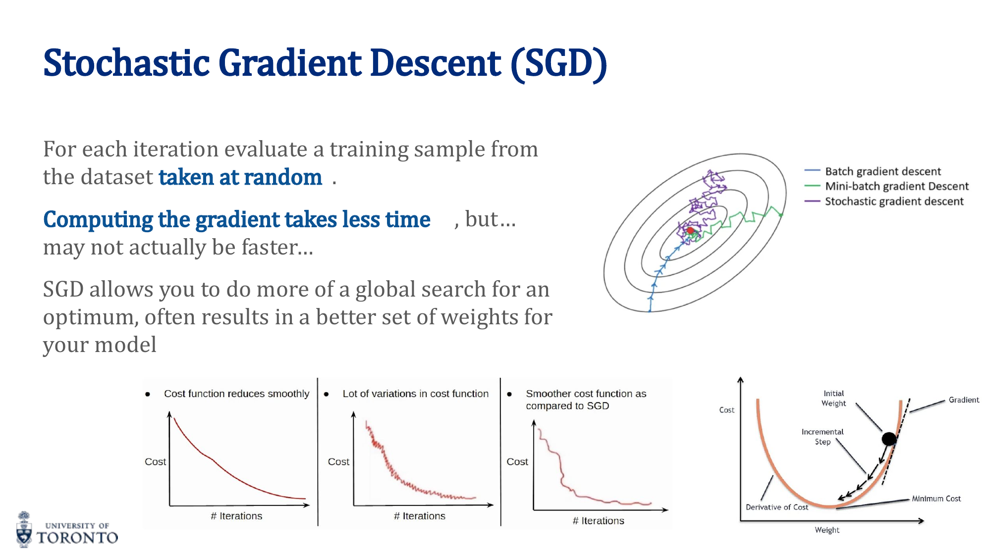
| Variant | Batch Size | Pros | Cons |
|---|---|---|---|
| SGD | 1 | Fast updates, can escape local minima | Very noisy, high variance |
| Mini-batch GD | n (e.g., 32-256) | Balanced noise/stability, GPU efficient | Requires tuning batch size |
| Batch GD | All samples | Stable convergence, low variance | Slow, memory expensive, stuck in local minima |
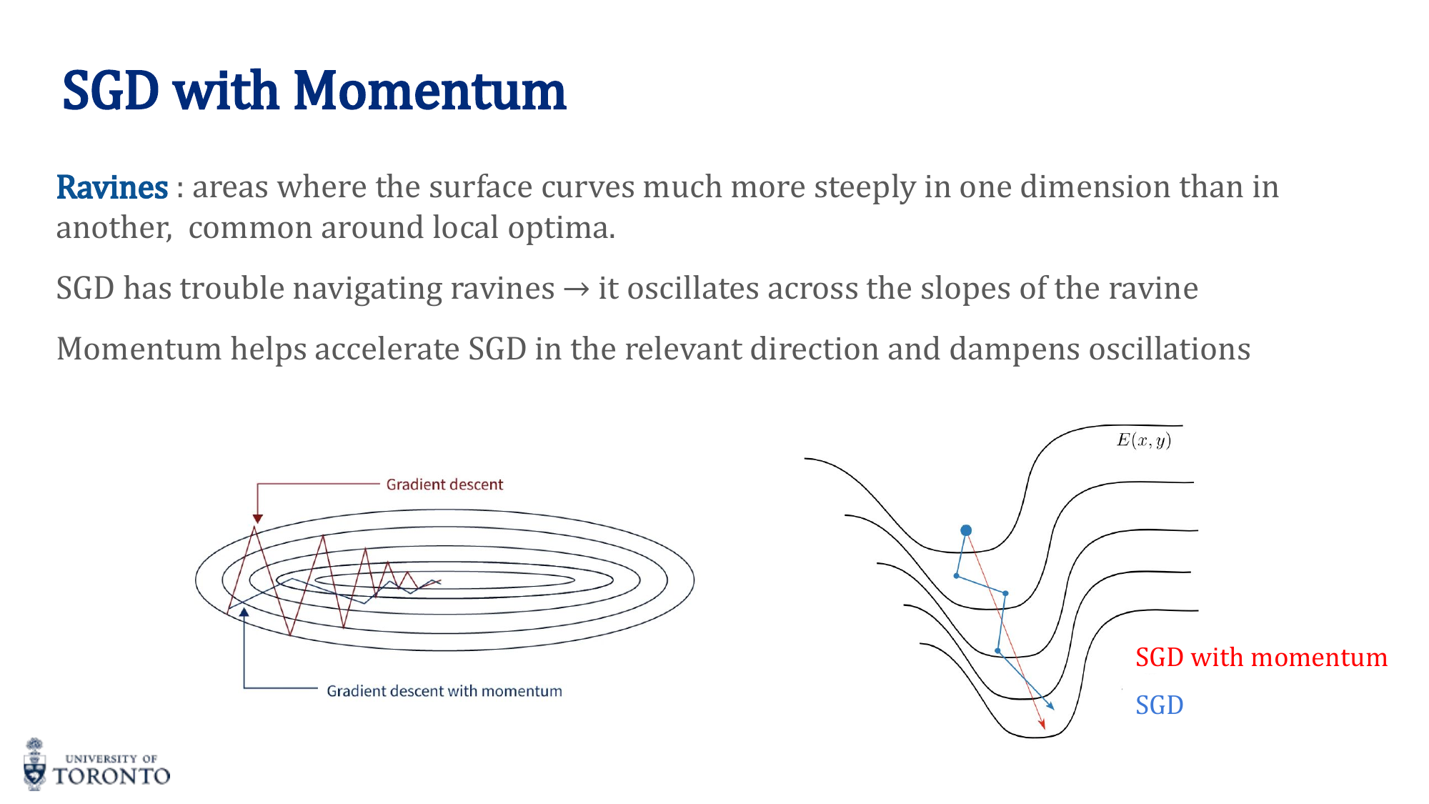
SGD with Momentum
Momentum accumulates a "velocity" from past gradients to smooth out oscillations and accelerate convergence:
w_(t+1) = w_t + v_t
Where λ is the momentum coefficient (typically 0.9). Think of a ball rolling down a hill — it builds up speed and can roll past small bumps.
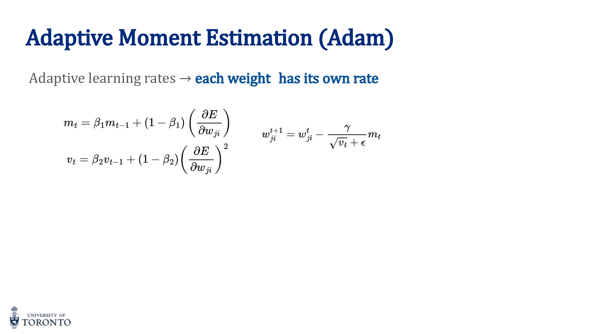
Adam Optimizer
Adam (Adaptive Moment Estimation) is the most commonly used optimizer. It combines momentum with adaptive per-parameter learning rates:
- Tracks first moment (mean of gradients) — like momentum
- Tracks second moment (variance of gradients) — adaptive rate
- Each weight gets its own learning rate based on its gradient history
- Includes bias correction for initial estimates
Key Insight
When in doubt, use Adam. It works well with default hyperparameters (lr=0.001, β1=0.9, β2=0.999) and requires minimal tuning. SGD with momentum can sometimes generalize better but requires more careful learning rate scheduling.
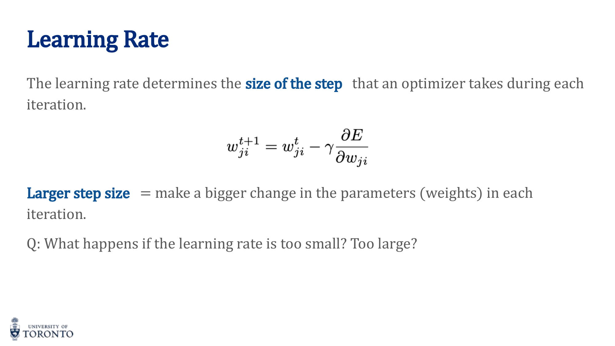
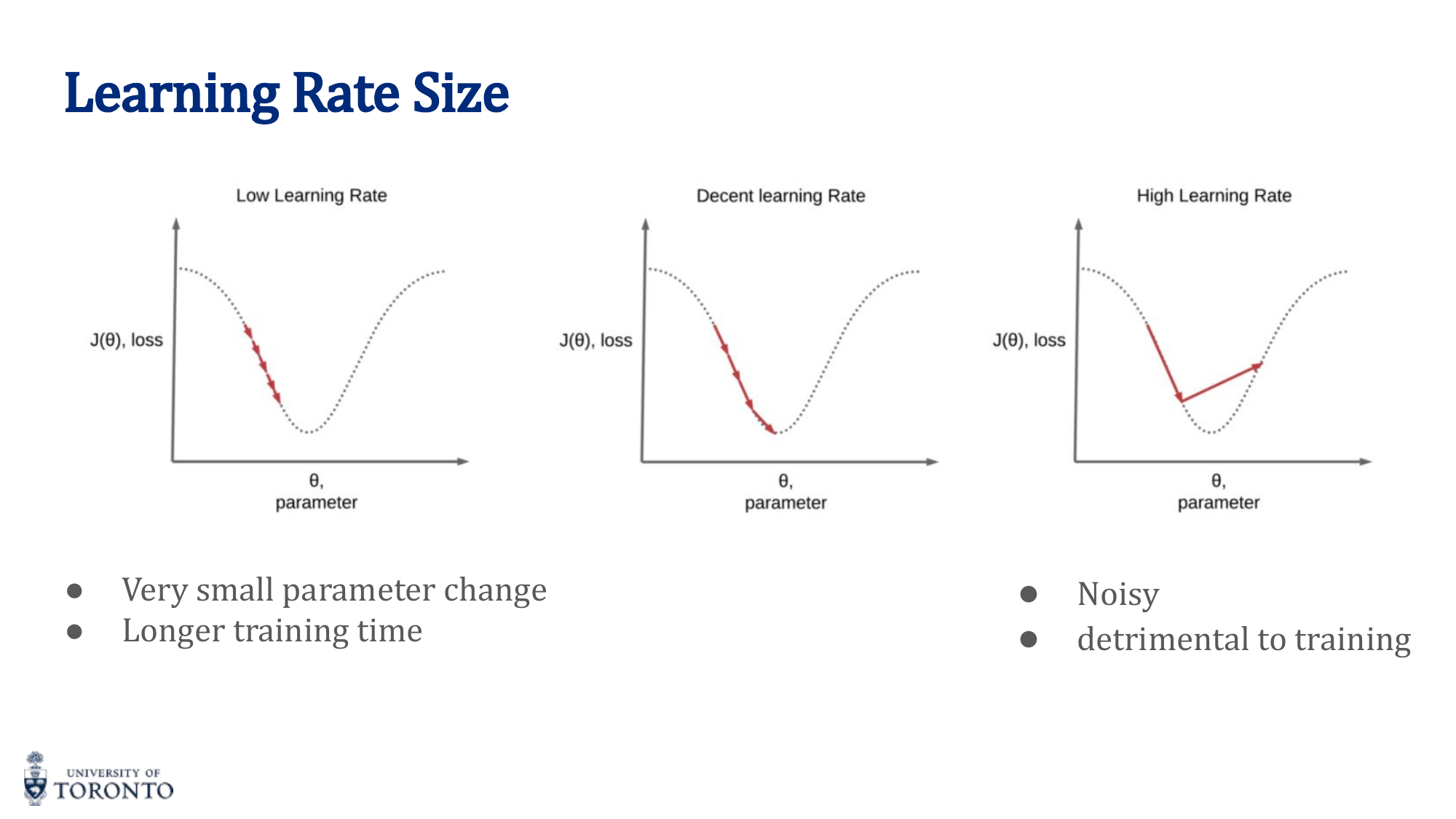
Learning Rate
The learning rate is arguably the most important hyperparameter:
- Too small: Training is extremely slow; may get stuck in suboptimal solutions
- Too large: Training is noisy, oscillates wildly, may diverge entirely
- Just right: Steady, consistent decrease in loss
Learning Rate Schedules: Reduce the learning rate during training for fine-grained convergence:
- Step Decay: Reduce by a factor every N epochs (e.g., halve every 10 epochs)
- Exponential Decay: lr_t = lr_0 · e^(-k·t)
- Cosine Annealing: Smoothly reduce following a cosine curve
Batch Size Tradeoffs
Batch size affects both training dynamics and generalization:
- Too small: Very noisy gradients, slow wall-clock time (can't leverage GPU parallelism)
- Too large: Expensive memory, tends to converge to sharp minima (worse generalization), fewer updates per epoch
- Sweet spot: Typically 32-256. Large enough for GPU efficiency, small enough for noise that helps generalization
Normalization
Input Normalization (Standardization): Scale inputs to zero mean and unit variance. Helps optimization by making the loss landscape more spherical.
Batch Normalization: Normalize activations within each mini-batch at each layer. Reduces internal covariate shift, allows higher learning rates, acts as mild regularization.
Regularization
Techniques to prevent overfitting (model memorizing training data):
- L2 Regularization (Weight Decay): Add
λ · ∑ w²to the loss. Penalizes large weights, pushes them toward zero. - L1 Regularization: Add
λ · ∑ |w|to the loss. Encourages sparsity (many weights become exactly zero). - Dropout: Randomly set a fraction of neurons to zero during training. Forces the network to not rely on any single neuron. Typical rate: 0.2-0.5.
- Early Stopping: Monitor validation loss; stop training when it begins to increase (overfitting starts).
- Data Augmentation: Artificially increase training data by applying transformations (flips, rotations, crops, color changes).
Evaluation Strategy
Data is split into three sets:
- Training set (~70-80%): Used to update weights
- Validation set (~10-15%): Used to tune hyperparameters and monitor overfitting
- Test set (~10-15%): Used ONCE for final evaluation. Never used to make decisions.
Overfitting: Low training loss, high validation loss. Model memorizes training data. Underfitting: High training loss, high validation loss. Model is too simple.
# PyTorch: Typical training setup with regularization
model = MyNetwork()
optimizer = torch.optim.Adam(model.parameters(), lr=1e-3, weight_decay=1e-4)
scheduler = torch.optim.lr_scheduler.StepLR(optimizer, step_size=10, gamma=0.5)

for epoch in range(num_epochs):
    model.train()
    for x_batch, y_batch in train_loader:
        output = model(x_batch)
        loss = criterion(output, y_batch)
        loss.backward()
        optimizer.step()
        optimizer.zero_grad()
    scheduler.step()

    model.eval()
    with torch.no_grad():
        val_loss = criterion(model(x_val), y_val)
    # Early stopping: if val_loss increases for N epochs, stop
Section III
Convolutional Neural Networks, Part I
Week 4 • Convolution, Filters & Feature Detection
Applying fully connected networks to images is impractical. A 256×256 color image has 196,608 input features; connecting each to even 1,000 hidden neurons yields nearly 200 million parameters in the first layer alone. Convolutional Neural Networks solve this by exploiting spatial structure: local connectivity, weight sharing, and translation equivariance.
Why Not Fully Connected?
- Too many parameters: Flattening images destroys spatial structure and creates an enormous number of weights
- Ignores geometry: Nearby pixels are more related than distant pixels, but FC networks treat all connections equally
- Not flexible: Trained on one image size, cannot handle a different size
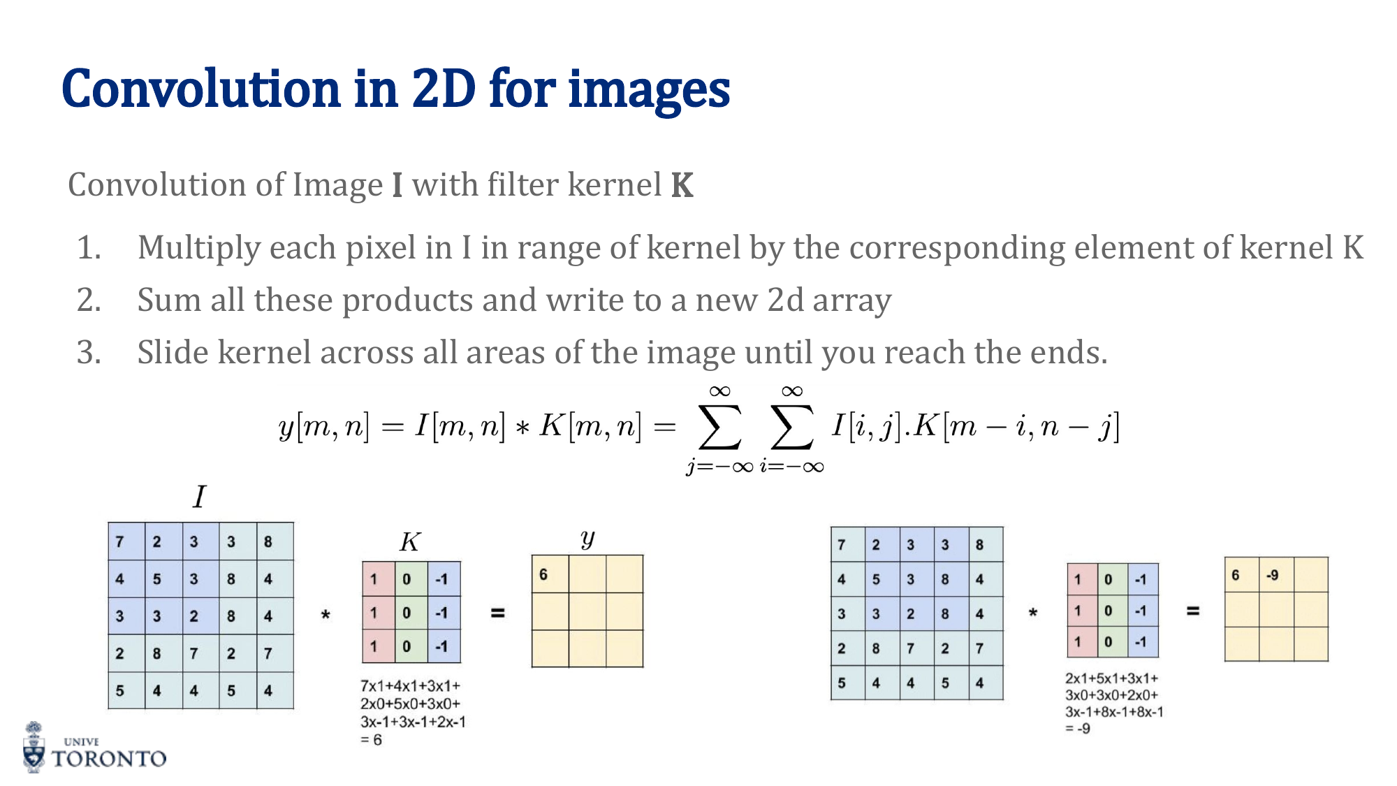
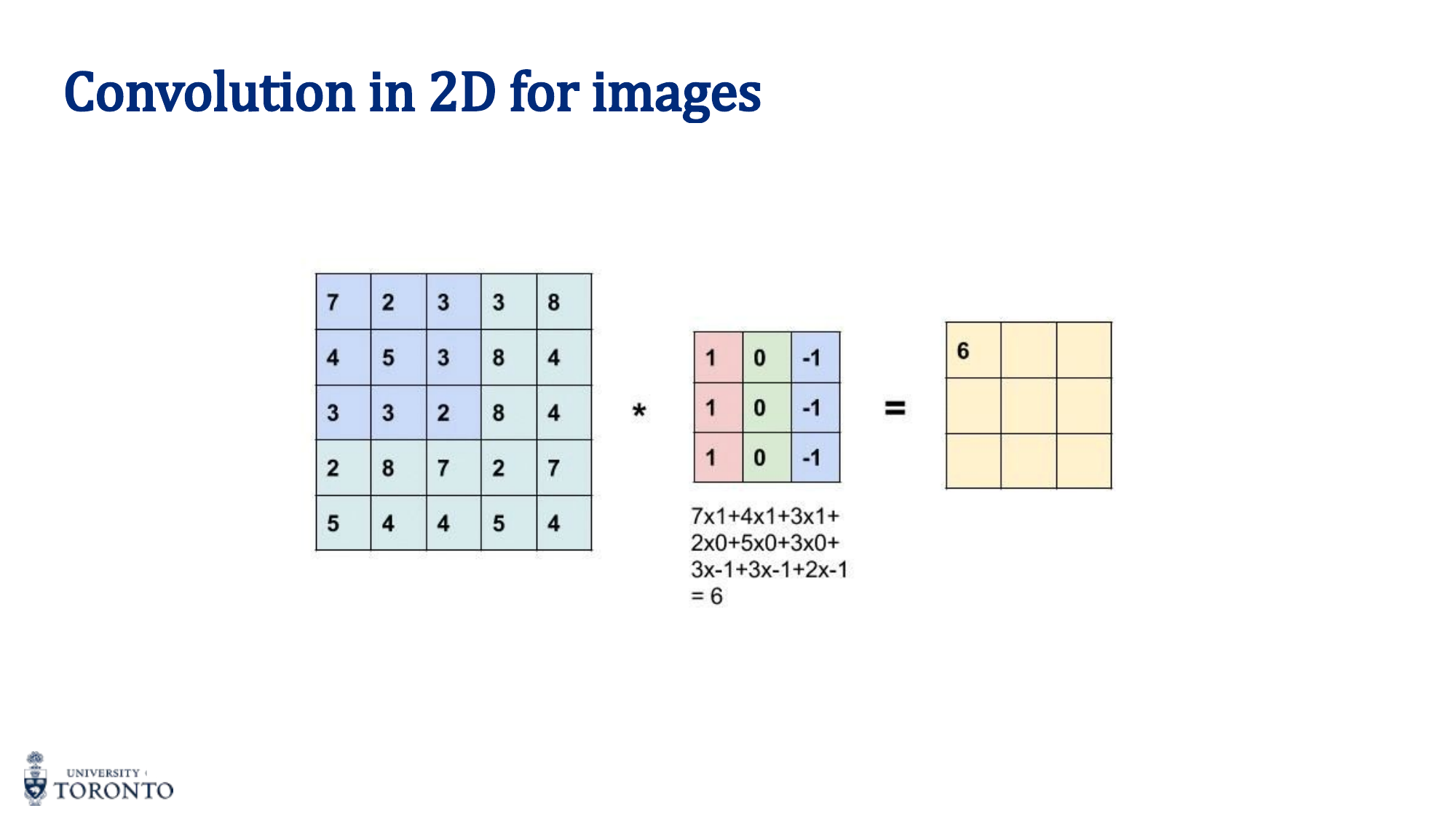
The Convolution Operation
A convolution slides a small filter (kernel) over the input, computing element-wise products and summing the results at each position. The filter acts as a feature detector.
Output Size Formula
Where n = input size, f = filter size, p = padding, s = stride.
Filter Types
Different kernels detect different features:
| Filter | Kernel | Detects |
|---|---|---|
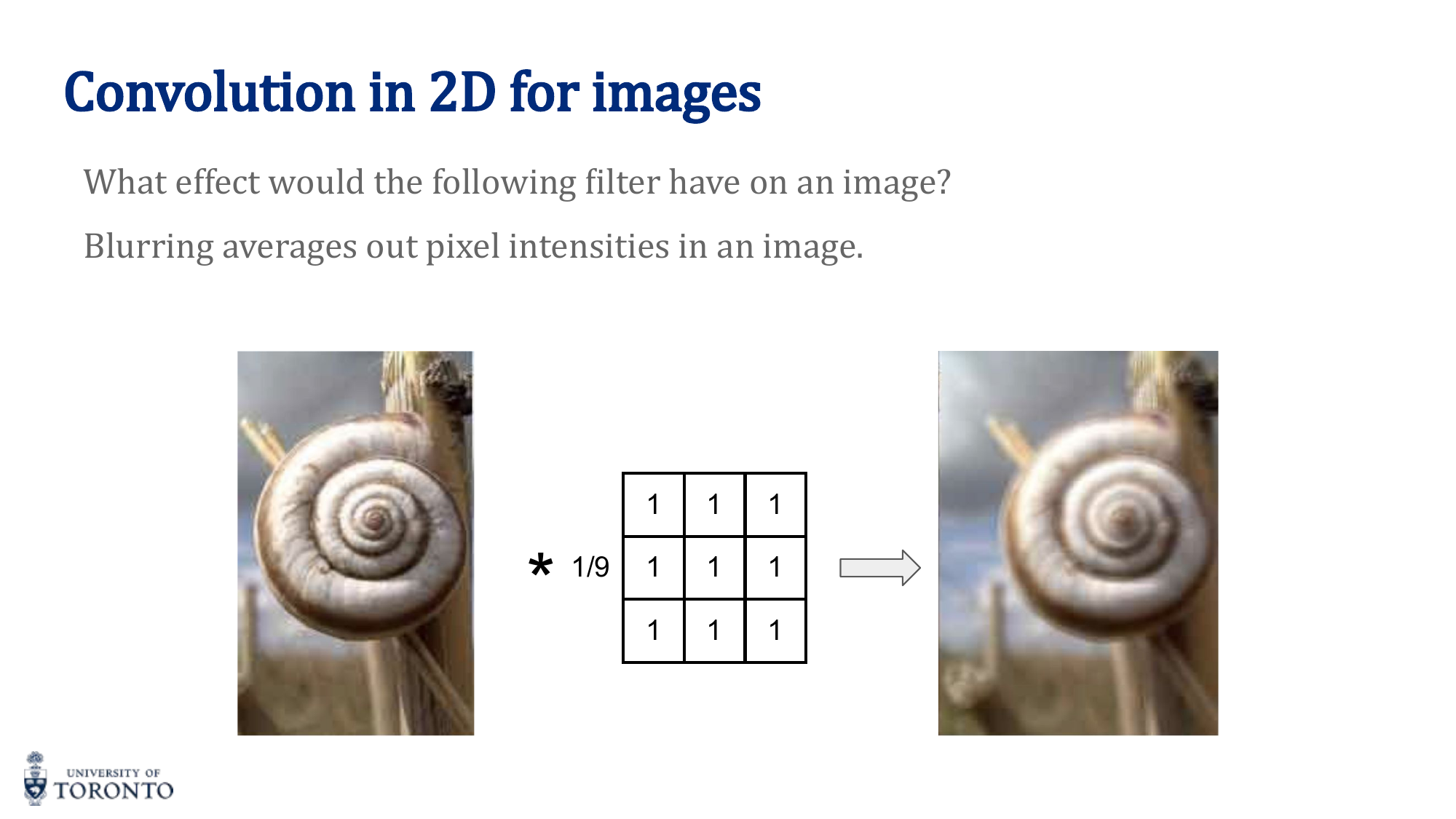
| Averaging | [[1/9]*9] | Blurring / smoothing |
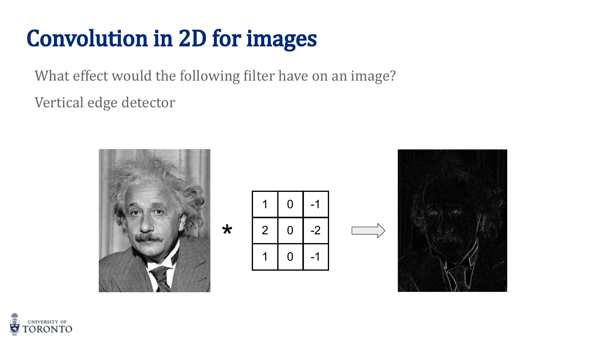
| Sobel Vertical | [1,0,-1; 2,0,-2; 1,0,-1] | Vertical edges |
| Sobel Horizontal | [1,2,1; 0,0,0; -1,-2,-1] | Horizontal edges |
| Laplacian | [0,1,0; 1,-4,1; 0,1,0] | Blobs / edges (second derivative) |
Stride and Padding
Stride: How many pixels the kernel moves between positions. Stride 1 = maximum overlap. Stride 2 = halves spatial dimensions.
Padding: Adding zeros around the border to control output size.
- "Valid" (no padding): Output shrinks. Output = (n - f)/s + 1
- "Same" padding: Output = input size. Requires p = (f - 1) / 2
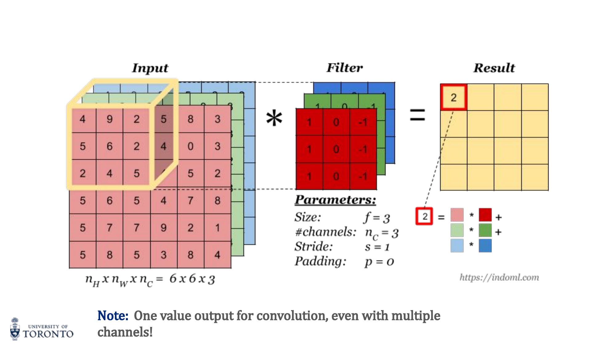
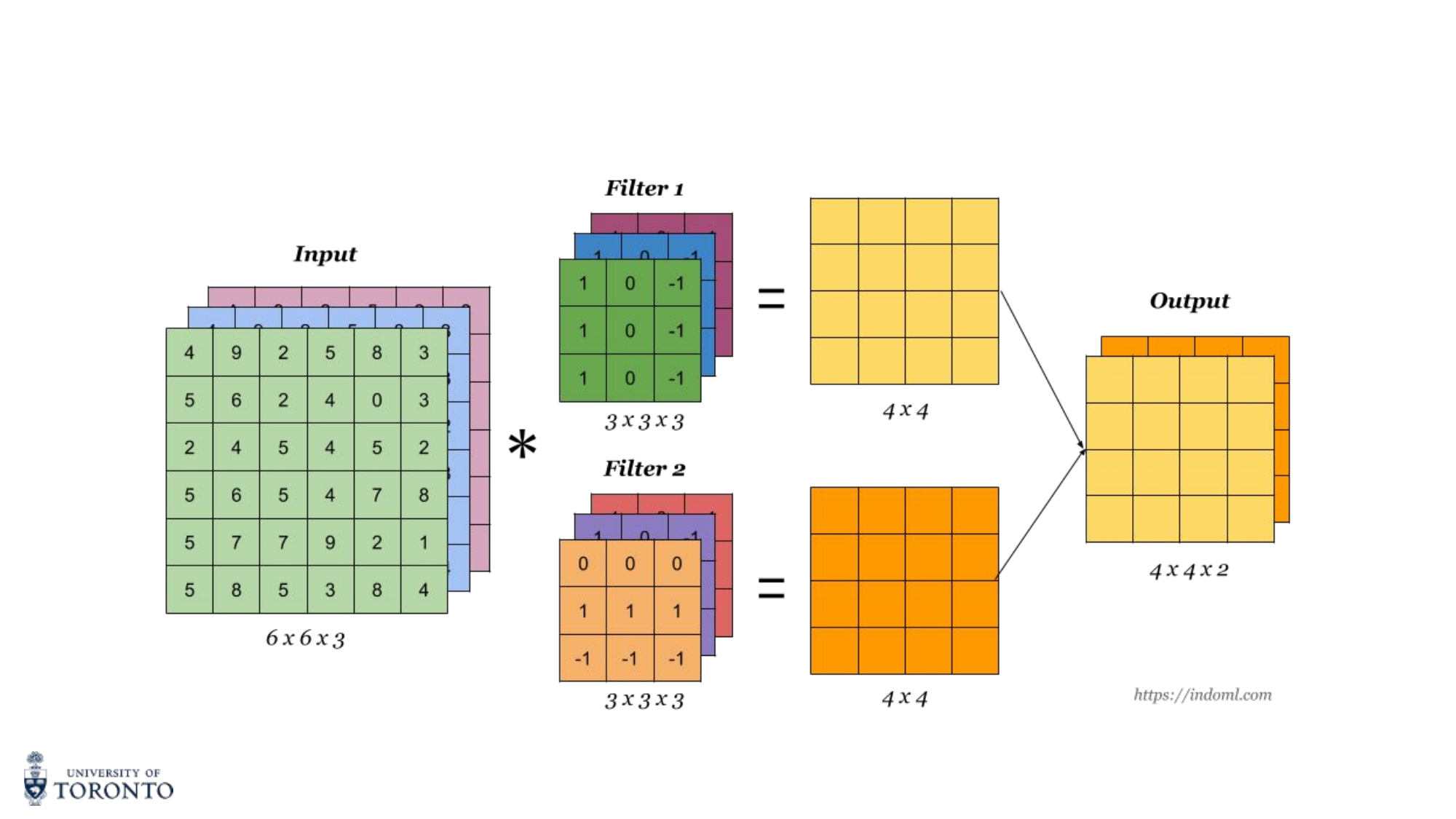
Multiple Channels
For RGB images (H × W × 3), the filter also has 3 channels. The convolution computes element-wise products across all channels and sums everything into a single 2D output. Multiple filters produce multiple output channels (feature maps).
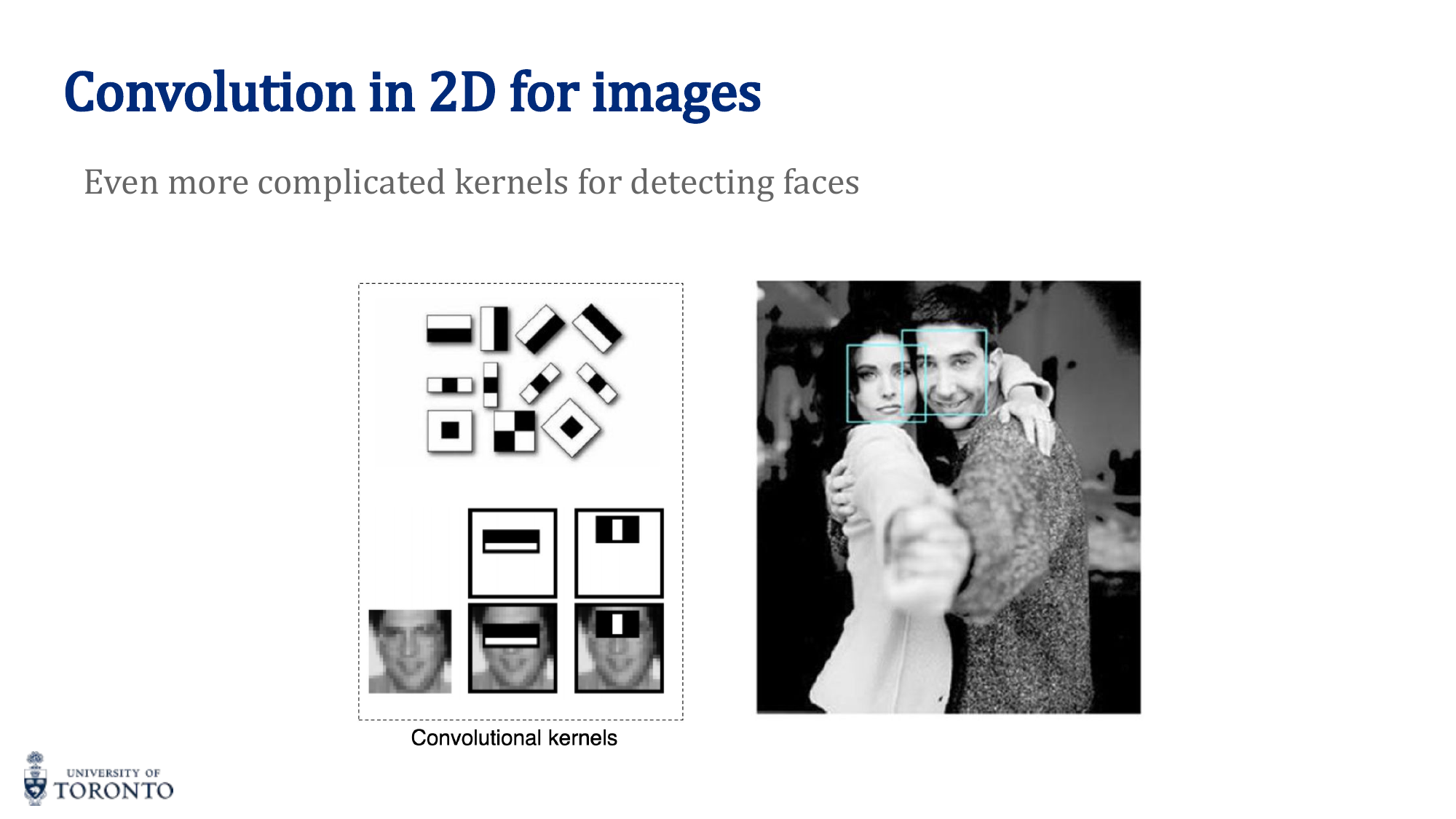
Key Insight
CNNs learn filters. Instead of hand-designing edge detectors or blob detectors, CNNs learn optimal filters through backpropagation. The network discovers what features matter for the task. Early layers learn simple edges, deeper layers learn complex patterns like textures and object parts.
# PyTorch: Convolution layers
import torch.nn as nn

# Input: batch of RGB images (B, 3, 32, 32)
conv1 = nn.Conv2d(in_channels=3, out_channels=16, kernel_size=3, stride=1, padding=1)
# Output: (B, 16, 32, 32) -- "same" padding preserves spatial dims

conv2 = nn.Conv2d(in_channels=16, out_channels=32, kernel_size=3, stride=2, padding=0)
# Output: (B, 32, 15, 15) -- stride=2 halves, no padding shrinks further

# Output size = (32 - 3 + 2*0) / 2 + 1 = 15
Section IV
Convolutional Neural Networks, Part II
Week 5 • Architectures, Transfer Learning & Visualization
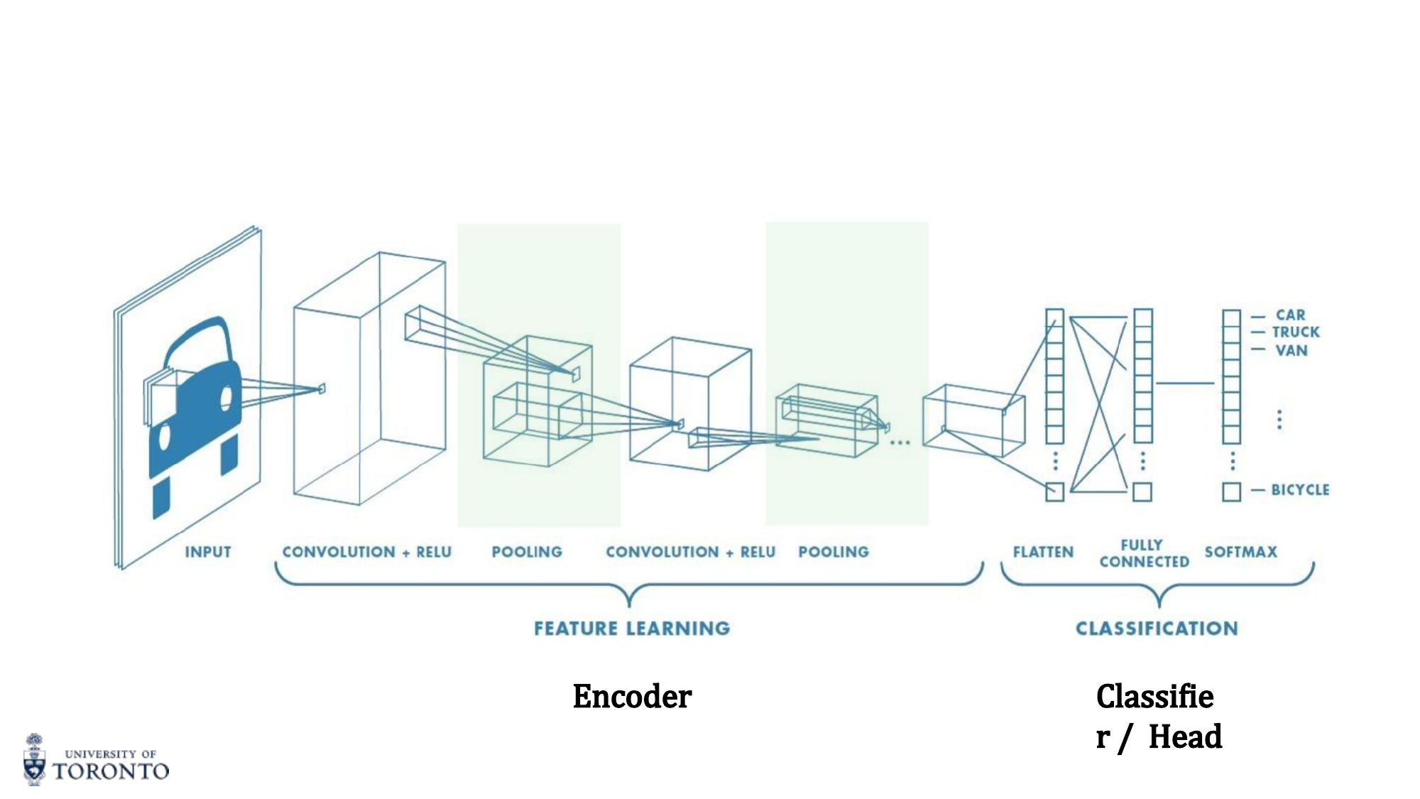
A complete CNN architecture consists of two parts: the encoder (feature extractor) that learns hierarchical representations through convolutional layers, and the classifier head that maps learned features to output predictions. Understanding landmark architectures and how to reuse them through transfer learning is essential for modern deep learning practice.
CNN Architecture Pipeline
The convolutional blocks form the encoder (feature learning). The fully connected layers form the classifier head. Pooling (max or average) reduces spatial dimensions progressively.
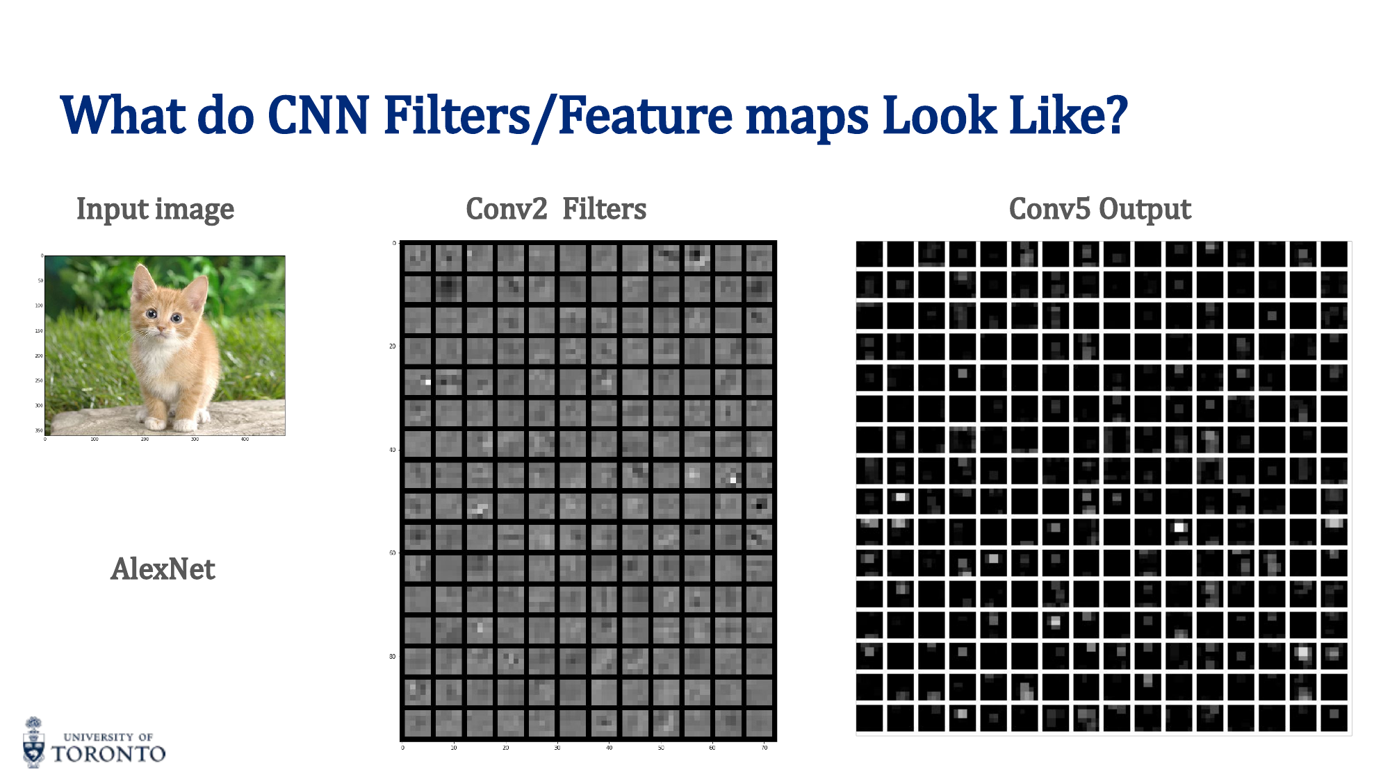
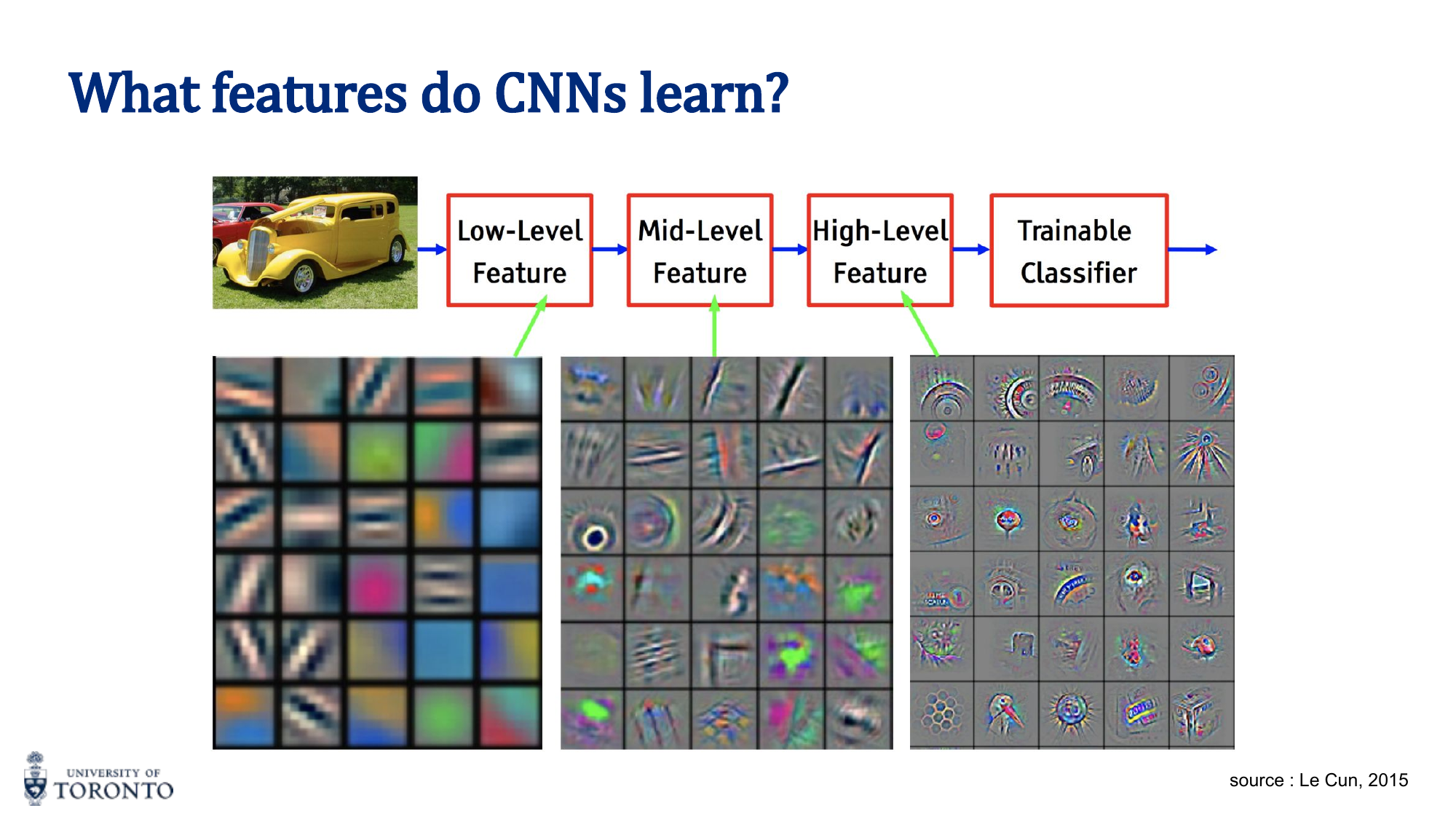
Visualizing CNN Features
What do CNNs actually learn? Visualization reveals a hierarchy:
- Early layers (Conv1, Conv2): Low-level features — edges, corners, color gradients
- Middle layers (Conv3, Conv4): Mid-level features — textures, patterns, parts of objects
- Deep layers (Conv5+): High-level features — object parts, faces, wheels, whole objects
Saliency Maps
Saliency maps compute the gradient of the output class score with respect to the input image pixels. High-gradient regions indicate which pixels most influenced the classification decision.
Landmark Architectures
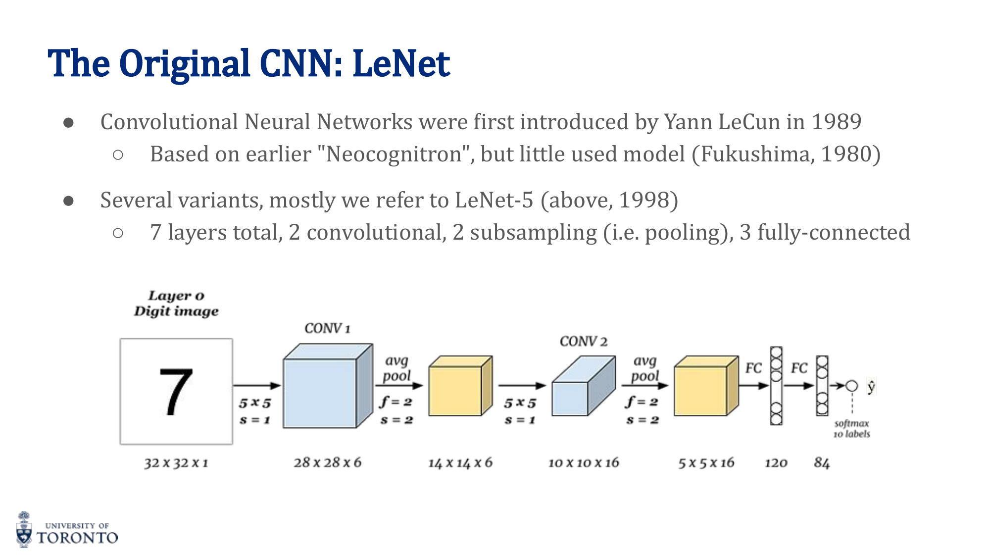
LeNet-5 (LeCun, 1989/1998)
The first successful CNN. Designed for handwritten digit recognition (MNIST). 7 layers: 2 convolutional + 2 pooling + 3 fully connected. Input: 32×32×1.
AlexNet (Krizhevsky et al., 2012)
The network that launched the deep learning revolution by winning ILSVRC 2012 with a ~10% improvement over the runner-up. Key innovations:
- Input: 227×227×3, approximately 60 million parameters
- First to use ReLU activation (instead of sigmoid/tanh)
- Dropout regularization
- Heavy data augmentation
- SGD with momentum, learning rate decay
- Trained on two GPUs (split architecture)
VGGNet (Simonyan & Zisserman, 2014)
Showed that depth matters. Uses only 3×3 filters throughout. VGG-16 (16 layers) and VGG-19 (19 layers) demonstrated that stacking small filters is more effective than using large ones.
ResNet (He et al., 2015)
Introduced skip connections (residual connections) that add the input of a block directly to its output:
This solves the degradation problem (deeper networks performing worse than shallower ones) by allowing gradients to flow directly through skip connections. Enables training networks with 100+ layers (ResNet-50, ResNet-101, ResNet-152).
Key Insight
Skip connections are revolutionary. Without them, very deep networks suffer from the degradation problem — not because of overfitting, but because optimization becomes too difficult. Residual connections let the network learn "corrections" to the identity mapping, making it easy for layers to learn the identity function if that's optimal.
Transfer Learning
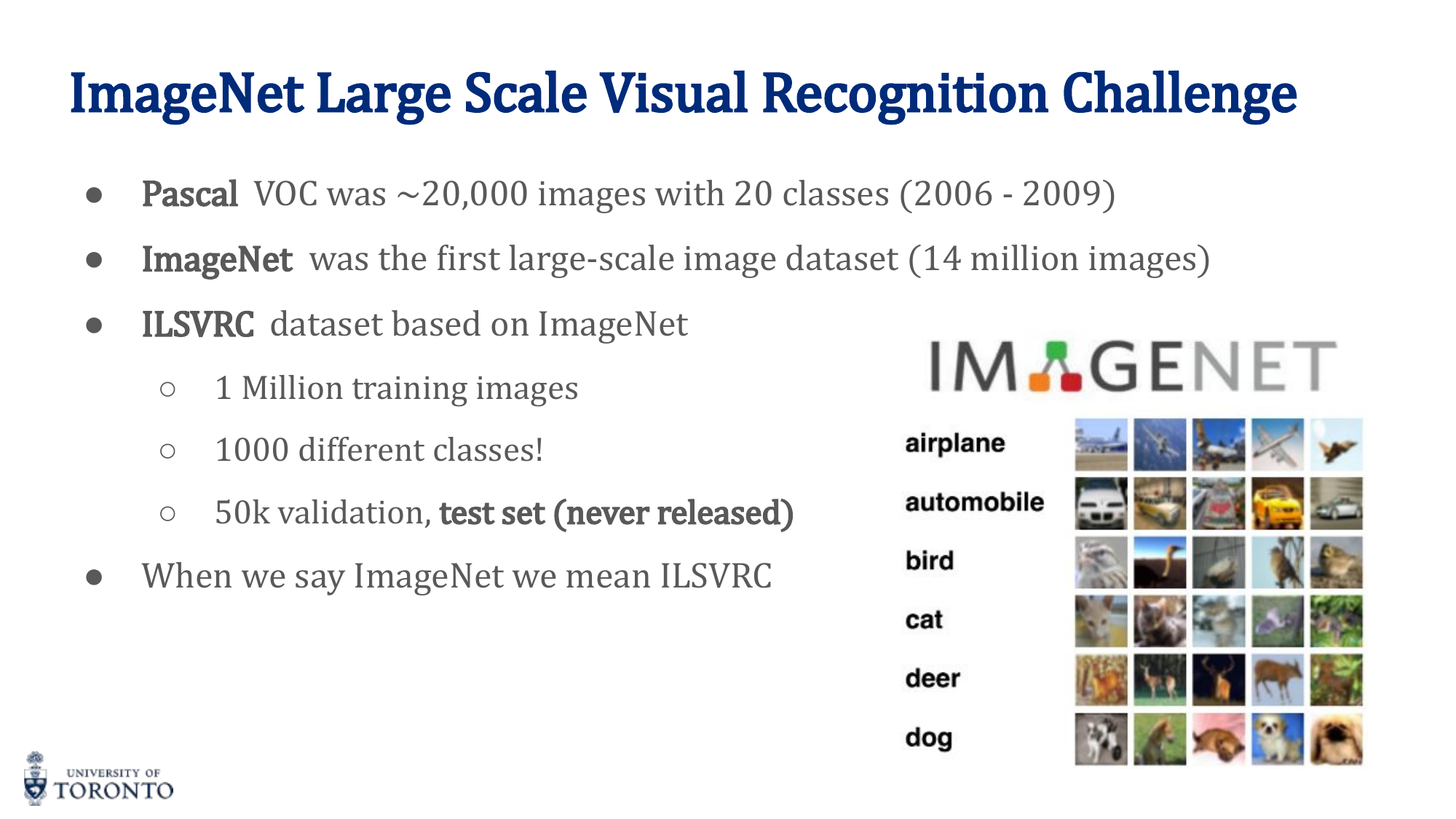
Instead of training from scratch, use a pre-trained model (e.g., trained on ImageNet with millions of images) and adapt it to your task:
- Feature Extraction: Freeze the encoder, replace and train only the classifier head. Fastest, works when your data is similar to the pre-training data.
- Fine-tuning: Unfreeze some or all encoder layers and train end-to-end with a small learning rate. Better when your data differs from pre-training data.
# PyTorch: Transfer Learning with ResNet
import torchvision.models as models

# Load pre-trained ResNet-18
model = models.resnet18(pretrained=True)

# Freeze encoder
for param in model.parameters():
    param.requires_grad = False

# Replace classifier head
model.fc = nn.Linear(512, num_classes)  # Only this layer trains

# For fine-tuning, unfreeze later layers:
# for param in model.layer4.parameters():
#     param.requires_grad = True
Data Augmentation
Artificially increase training data by applying random transformations:
- Random horizontal/vertical flips
- Random crops and resizing
- Color jittering (brightness, contrast, saturation)
- Random rotation
- Cutout / Random erasing
# PyTorch: Data Augmentation
from torchvision import transforms

train_transform = transforms.Compose([
    transforms.RandomHorizontalFlip(),
    transforms.RandomCrop(32, padding=4),
    transforms.ColorJitter(brightness=0.2, contrast=0.2),
    transforms.RandomRotation(15),
    transforms.ToTensor(),
    transforms.Normalize(mean=[0.485, 0.456, 0.406],
                         std=[0.229, 0.224, 0.225])
])
Section V
Unsupervised Learning
Week 6 • Autoencoders & Variational Autoencoders
Supervised learning requires labeled data, which is expensive and time-consuming to collect. Unsupervised learning discovers structure and patterns in data without labels. Autoencoders learn compressed representations by reconstructing their own input, while Variational Autoencoders extend this idea to generate new, realistic data by learning smooth, continuous latent spaces.
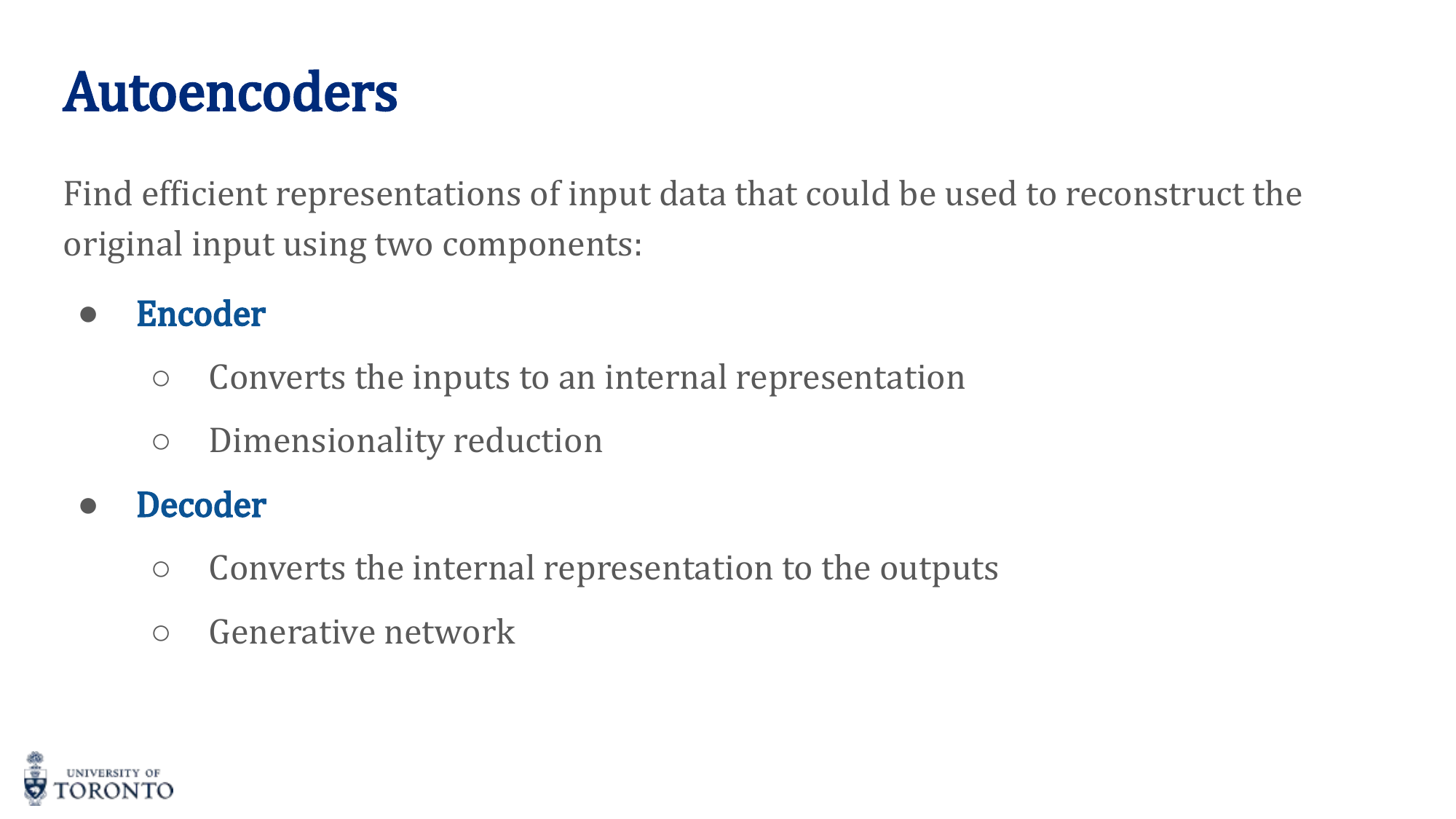
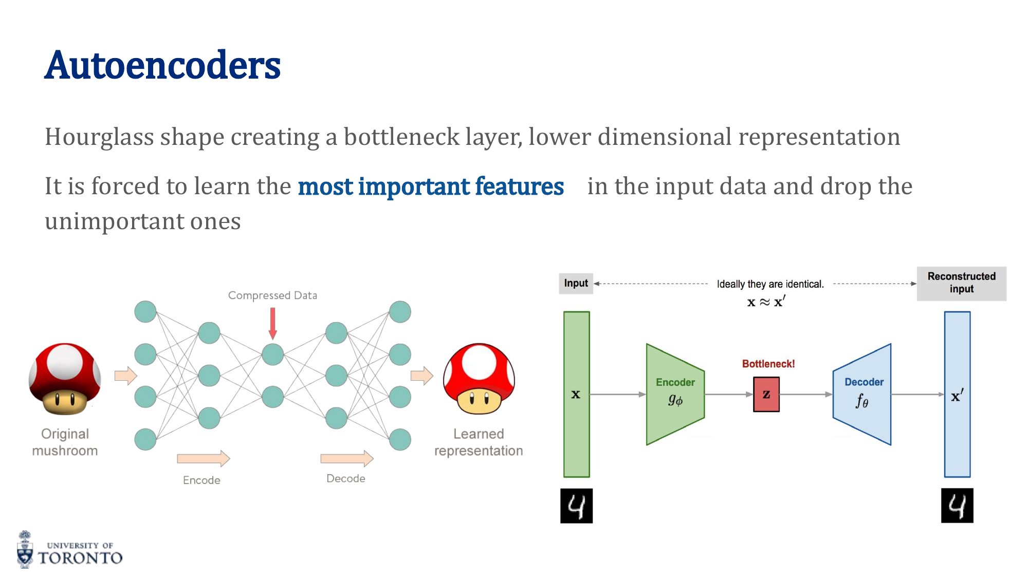
Autoencoders
An autoencoder has two parts:
- Encoder: Compresses input to a low-dimensional latent representation (bottleneck)
- Decoder: Reconstructs the original input from the latent representation
The hourglass shape forces the network to learn the most important features of the data — it cannot simply copy the input through the bottleneck.
Training Autoencoders
The loss function is reconstruction loss — MSE between input and output:
Crucially, the input IS the target. The network learns an identity function, but constrained by the bottleneck to capture only the most salient features.
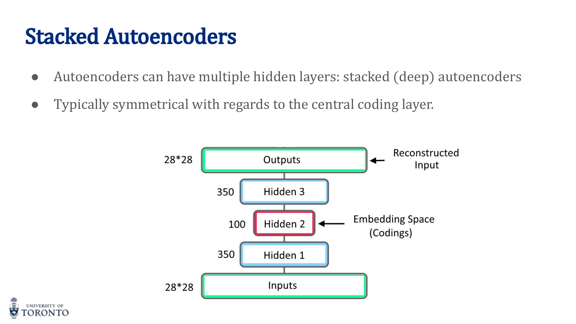
Stacked Autoencoders
Multiple hidden layers in both encoder and decoder, typically symmetrical. Deeper autoencoders can learn more complex, hierarchical representations.
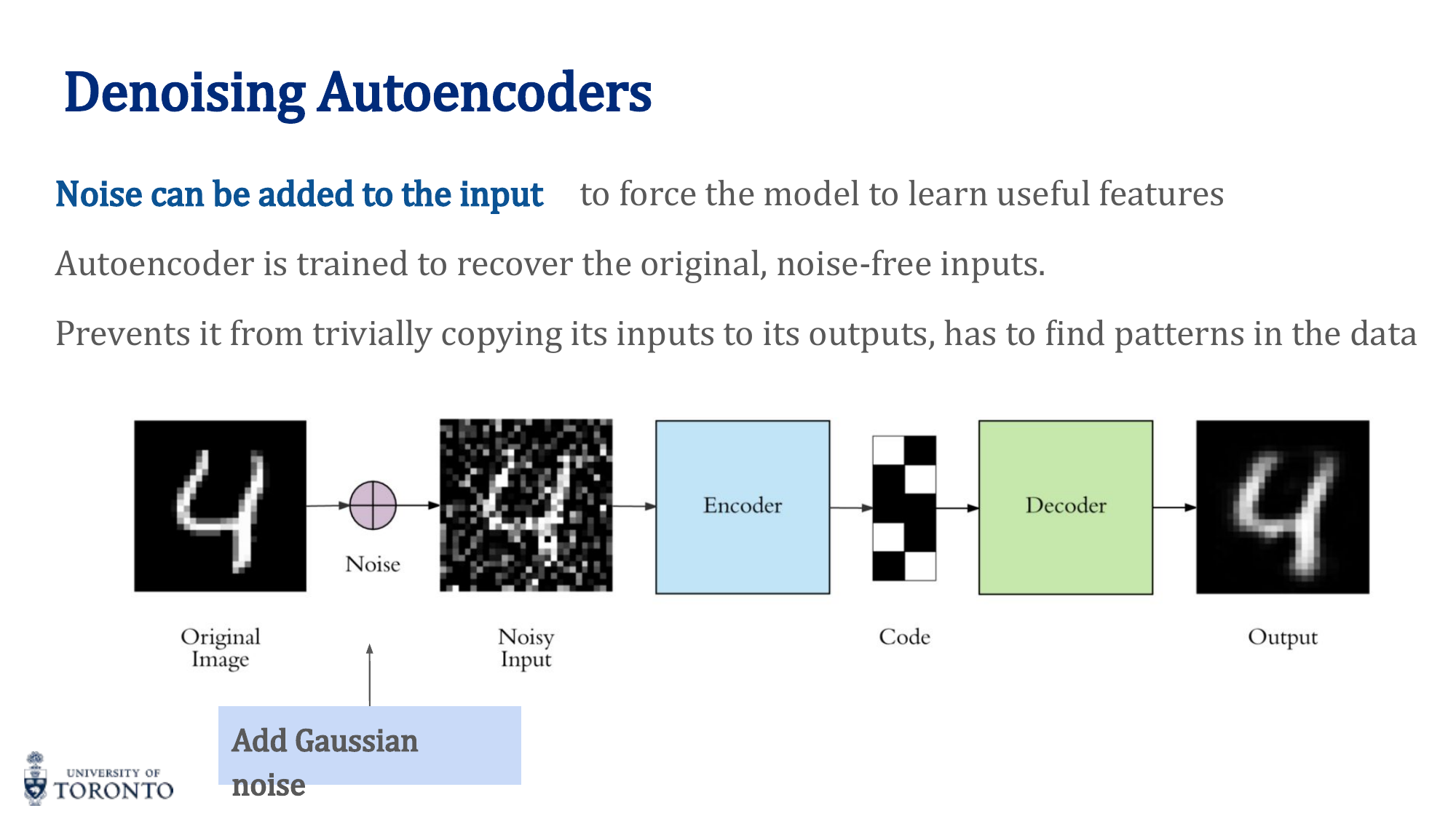
Denoising Autoencoders
Add Gaussian noise to the input but train to reconstruct the clean original. This prevents the network from learning a trivial identity mapping and forces it to capture robust features.
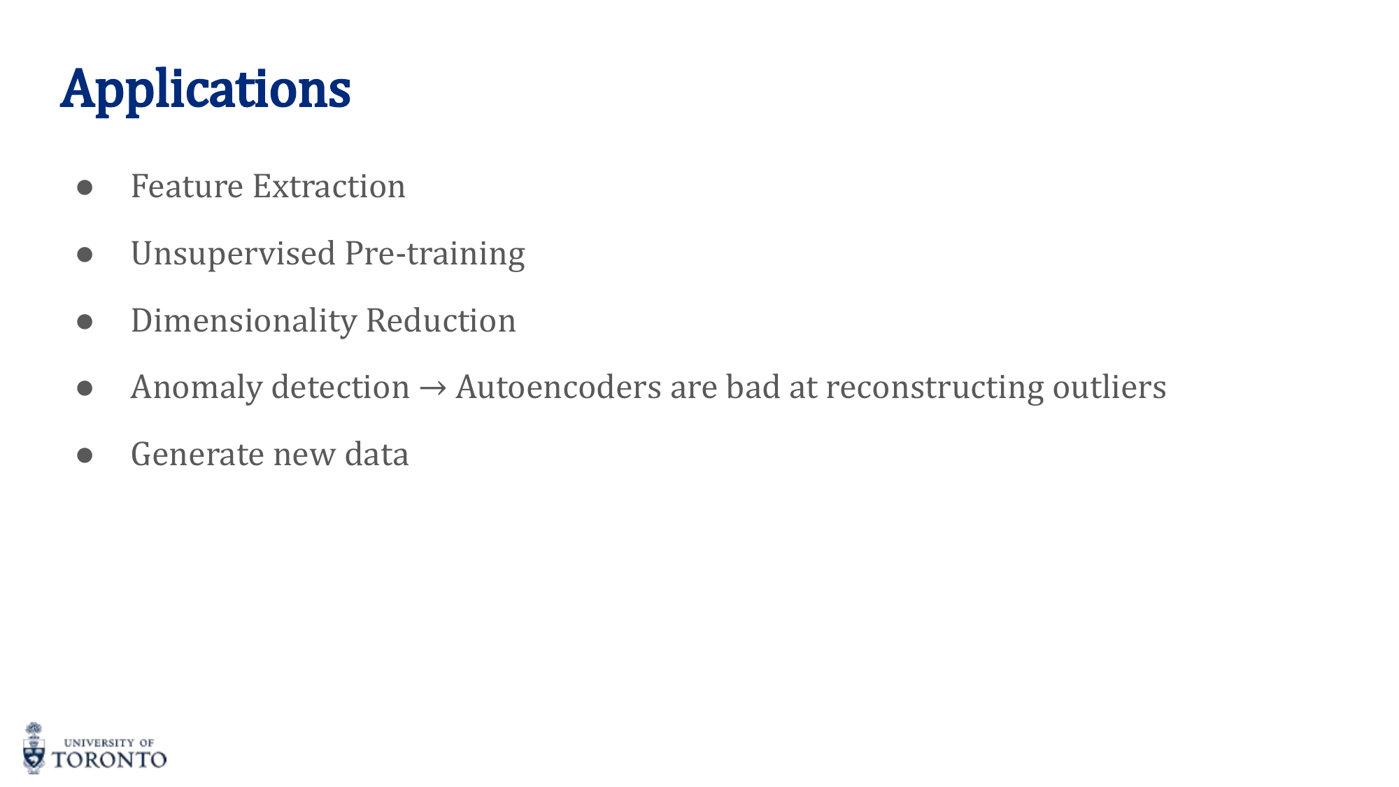
Applications of Autoencoders
- Feature extraction: Use the encoder's bottleneck representation as features for downstream tasks
- Dimensionality reduction: Non-linear alternative to PCA
- Anomaly detection: Normal data reconstructs well; anomalies have high reconstruction error
- Data generation: Sample from latent space, decode to generate new data
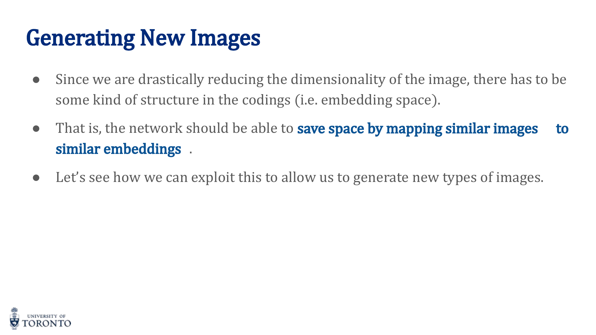
Generating Images via Interpolation
Encode two images to get their latent vectors, linearly interpolate between them, and decode the intermediate points to produce smooth transitions between images.
The Problem with Standard Autoencoders
Standard autoencoders produce latent spaces that can be disjoint and non-continuous. Random sampling from such a space produces garbage output because there are "holes" where no training data maps.
Variational Autoencoders (VAE)
VAEs solve the generation problem by making the latent space smooth and continuous:
- The encoder outputs a distribution (mean μ and variance σ²) rather than a single point
- A sample is drawn from this distribution: z ~ N(μ, σ²)
- KL divergence loss regularizes the distribution to be close to a standard normal N(0, 1)
VAE Loss Function
L = MSE(x, x̂) + D_KL(q(z|x) || p(z))
The reconstruction loss ensures the output looks like the input. The KL divergence regularizes the latent space to be smooth and close to N(0, 1), enabling meaningful interpolation and random sampling.
Reparameterization Trick
Sampling is a non-differentiable operation. The reparameterization trick makes it differentiable:
The randomness is isolated in ε (which doesn't depend on parameters), so gradients can flow through μ and σ during backpropagation.
Key Insight
VAE = Autoencoder + Probabilistic Latent Space. The key innovation is forcing the encoder to output distributions and regularizing them with KL divergence. This creates a smooth, continuous latent space where nearby points decode to similar outputs, enabling both generation (random sampling) and meaningful interpolation.
# PyTorch: VAE
class VAE(nn.Module):
    def __init__(self, input_dim, latent_dim):
        super().__init__()
        self.encoder = nn.Sequential(
            nn.Linear(input_dim, 256), nn.ReLU(),
            nn.Linear(256, 128), nn.ReLU())
        self.fc_mu = nn.Linear(128, latent_dim)
        self.fc_logvar = nn.Linear(128, latent_dim)
        self.decoder = nn.Sequential(
            nn.Linear(latent_dim, 128), nn.ReLU(),
            nn.Linear(128, 256), nn.ReLU(),
            nn.Linear(256, input_dim), nn.Sigmoid())

    def reparameterize(self, mu, logvar):
        std = torch.exp(0.5 * logvar)
        eps = torch.randn_like(std)       # epsilon ~ N(0,1)
        return mu + std * eps             # z = mu + sigma * eps

    def forward(self, x):
        h = self.encoder(x)
        mu, logvar = self.fc_mu(h), self.fc_logvar(h)
        z = self.reparameterize(mu, logvar)
        return self.decoder(z), mu, logvar

# VAE Loss
def vae_loss(x_recon, x, mu, logvar):
    recon = nn.functional.mse_loss(x_recon, x, reduction='sum')
    kl = -0.5 * torch.sum(1 + logvar - mu.pow(2) - logvar.exp())
    return recon + kl
Section VI
Recurrent Neural Networks, Part I
Week 7 • Word Embeddings: word2vec & GloVe
Before we can process text with neural networks, we need to represent words as numbers. One-hot encoding creates sparse, high-dimensional vectors with no notion of similarity. Word embeddings solve this by learning dense, low-dimensional vectors where semantically similar words are close together in the vector space.
The Problem with One-Hot Encoding
With a vocabulary of 50,000 words, each word is a 50,000-dimensional vector with a single 1. Problems:
- Extremely high-dimensional and sparse
- No notion of similarity: "cat" and "kitten" are as different as "cat" and "airplane"
- Every word is equidistant from every other word
Word Embeddings
Learned dense vectors (typically 50-300 dimensions) where:
- Similar words have similar vectors (small distance/high cosine similarity)
- Semantic relationships are captured: king - man + woman ≈ queen
- Trained on large text corpora in an unsupervised manner
word2vec
A family of architectures for learning word embeddings from text. Two main variants:
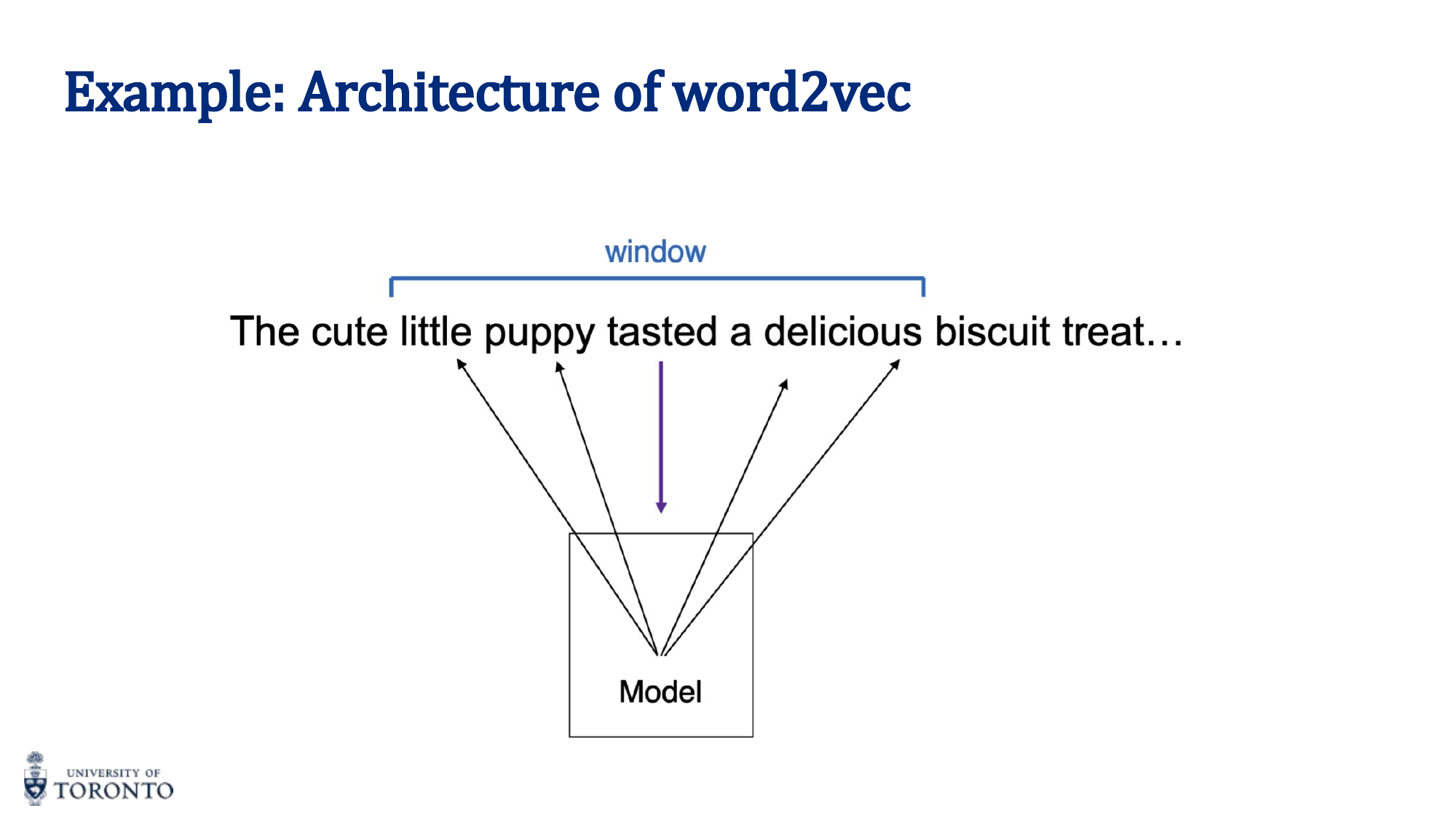
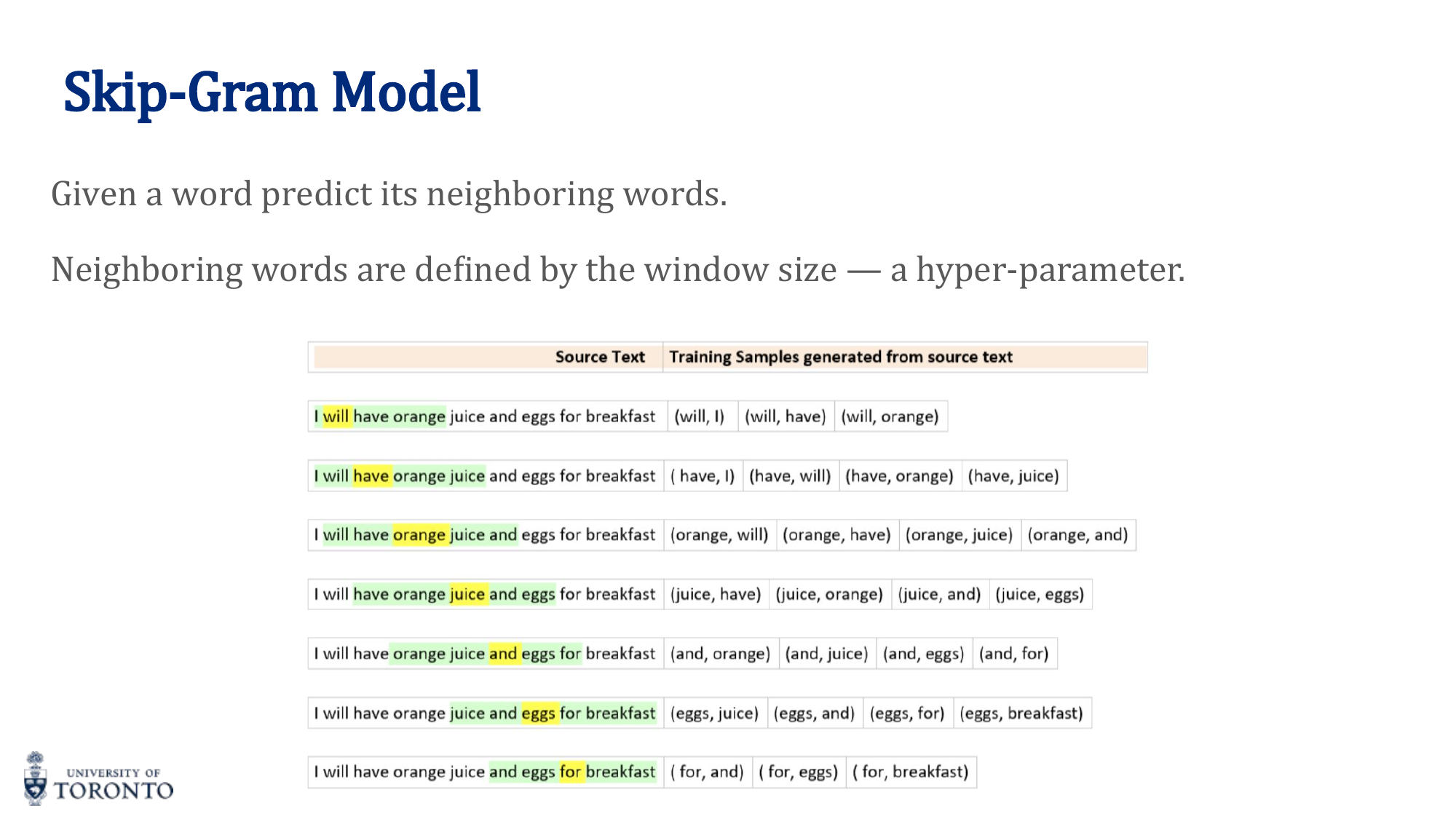
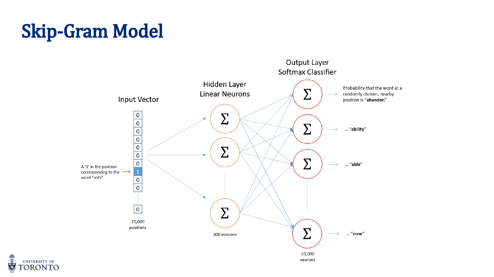
Skip-Gram
Given a center (target) word, predict the surrounding context words within a window. The training creates (center, context) pairs:
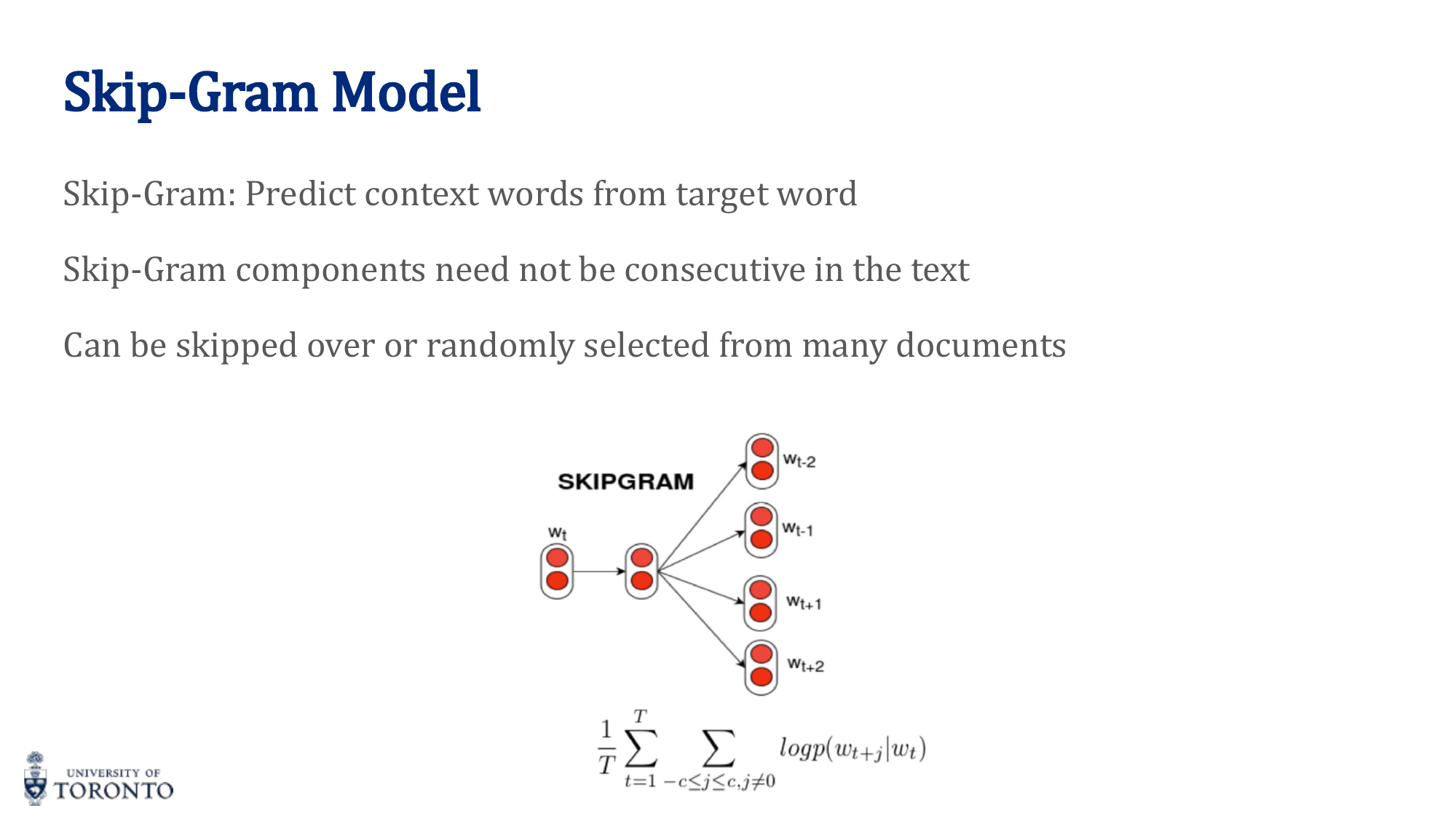
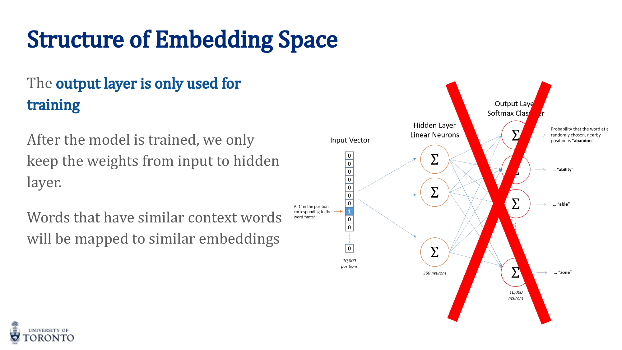
After training, only the encoder (input-to-hidden) weights are kept. These weights ARE the word embeddings.
CBOW (Continuous Bag of Words)
The reverse: given the context words, predict the center word. Generally faster to train, better for frequent words.
| Property | CBOW | Skip-Gram |
|---|---|---|
| Input | Context words | Center word |
| Output | Center word | Context words |
| Speed | Faster training | Slower training |
| Rare words | Worse | Better |
GloVe (Global Vectors)
Unlike word2vec (which uses local context windows), GloVe uses global co-occurrence statistics. It constructs a co-occurrence matrix from the entire corpus and learns embeddings where:
Where X_ij is the co-occurrence count of words i and j. The inner product of word vectors approximates the logarithm of their co-occurrence frequency.
Distance Measures
- Euclidean Distance (L2 norm):
d(a,b) = sqrt(∑(a_i - b_i)²). Affected by vector magnitude. - Cosine Similarity:
cos(a,b) = (a · b) / (||a|| · ||b||). Measures the angle between vectors. Invariant to magnitude. Range: [-1, 1]. Preferred for word embeddings because it measures directional similarity.
Key Insight
Cosine similarity is preferred for word embeddings because we care about the direction (semantic meaning) of vectors, not their magnitude. Two vectors pointing in the same direction are similar regardless of their length. Euclidean distance can be misleading when vectors have different magnitudes.
# PyTorch: Using pre-trained embeddings
import torch.nn as nn

# Embedding layer: lookup table mapping word indices to vectors
embedding = nn.Embedding(num_embeddings=vocab_size, embedding_dim=300)

# Using pre-trained GloVe
# embedding.weight = nn.Parameter(glove_vectors)
# embedding.weight.requires_grad = False  # Freeze if using as fixed features

# Cosine similarity
cos_sim = nn.CosineSimilarity(dim=1)
similarity = cos_sim(embedding(word1_idx), embedding(word2_idx))
Section VII
Recurrent Neural Networks, Part II
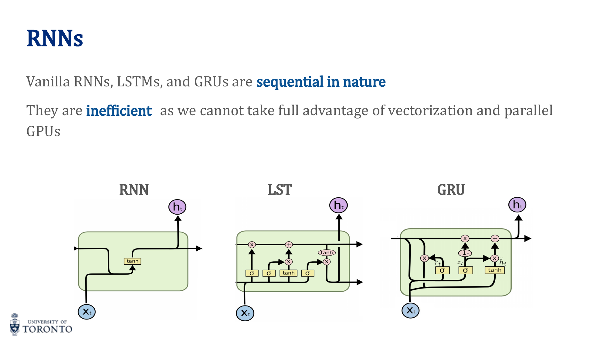
Week 8 • RNNs, LSTMs & GRUs
Many real-world problems involve sequential data: time series, natural language, audio, video. Unlike feedforward networks that process fixed-size inputs, Recurrent Neural Networks maintain a hidden state that captures information from previous time steps, enabling them to handle variable-length sequences. However, standard RNNs struggle with long-range dependencies, leading to the development of gated architectures like LSTM and GRU.
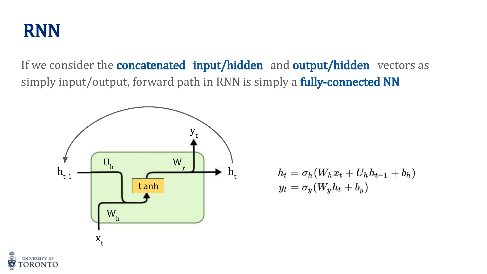
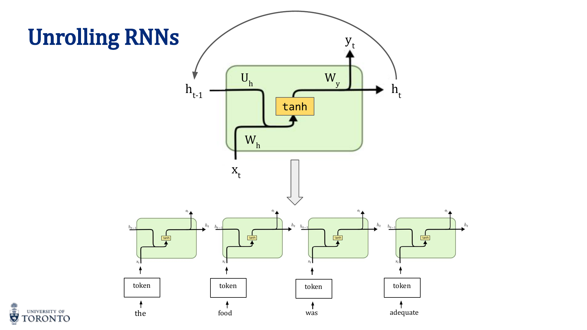
RNN Architecture
An RNN applies the same neural network at each time step, maintaining a hidden state that carries information forward:
y_t = σ_y(W_y · h_t + b_y)
The hidden state h_t is a function of both the current input x_t and the previous hidden state h_(t-1). Weights are shared across all time steps.
RNN Types by Input/Output
| Type | Input | Output | Example |
|---|---|---|---|
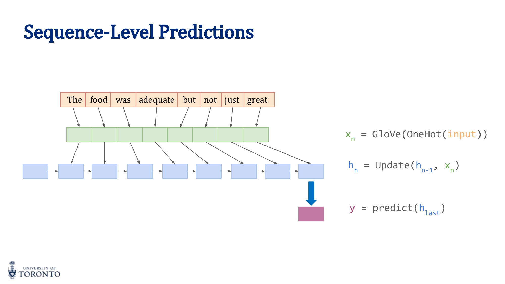
| Many-to-One | Sequence | Single label | Sentiment analysis, text classification |
| One-to-Many | Single input | Sequence | Image captioning, music generation |
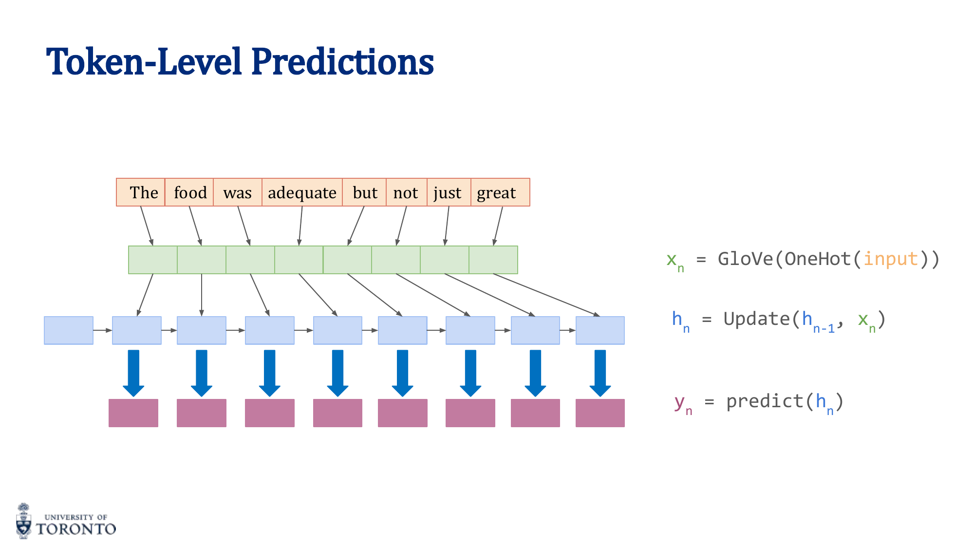
| Many-to-Many (same length) | Sequence | Sequence | POS tagging, named entity recognition |
| Many-to-Many (diff length) | Sequence | Sequence | Machine translation (encoder-decoder) |
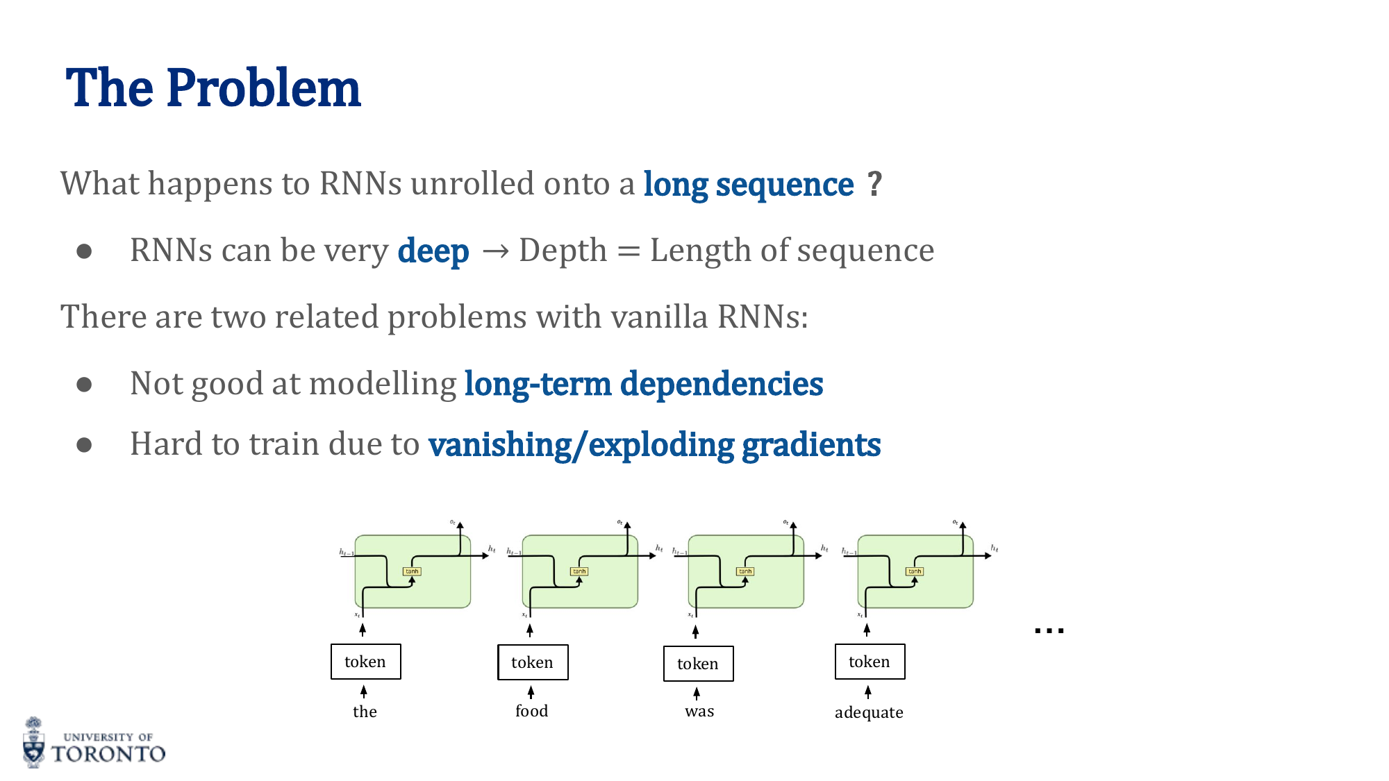
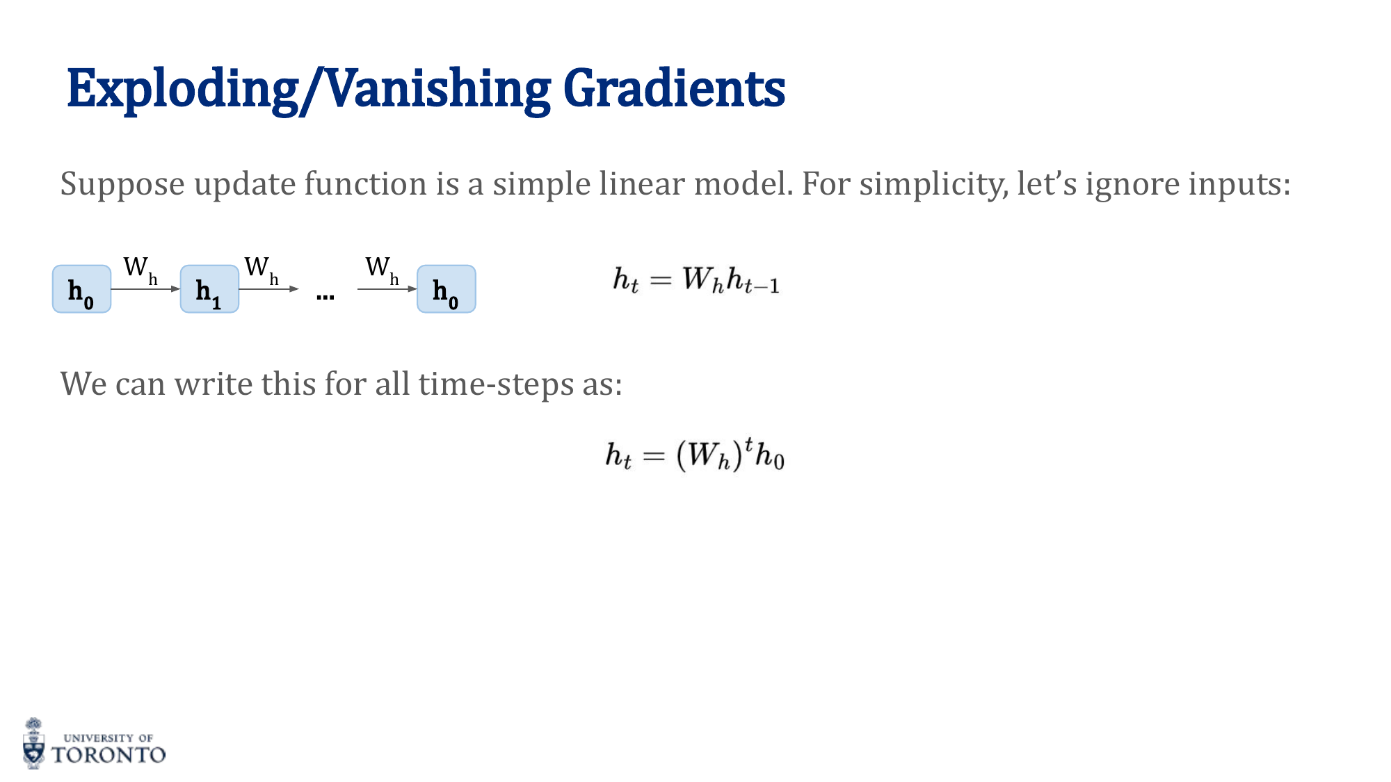
Vanishing and Exploding Gradients
During backpropagation through time, gradients are multiplied by the weight matrix W_h at each step:
If the largest eigenvalue of W_h is greater than 1, gradients explode. If less than 1, gradients vanish. This means standard RNNs cannot effectively learn long-range dependencies.
Solutions:
- Gradient clipping (for exploding): Cap the gradient norm to a maximum value
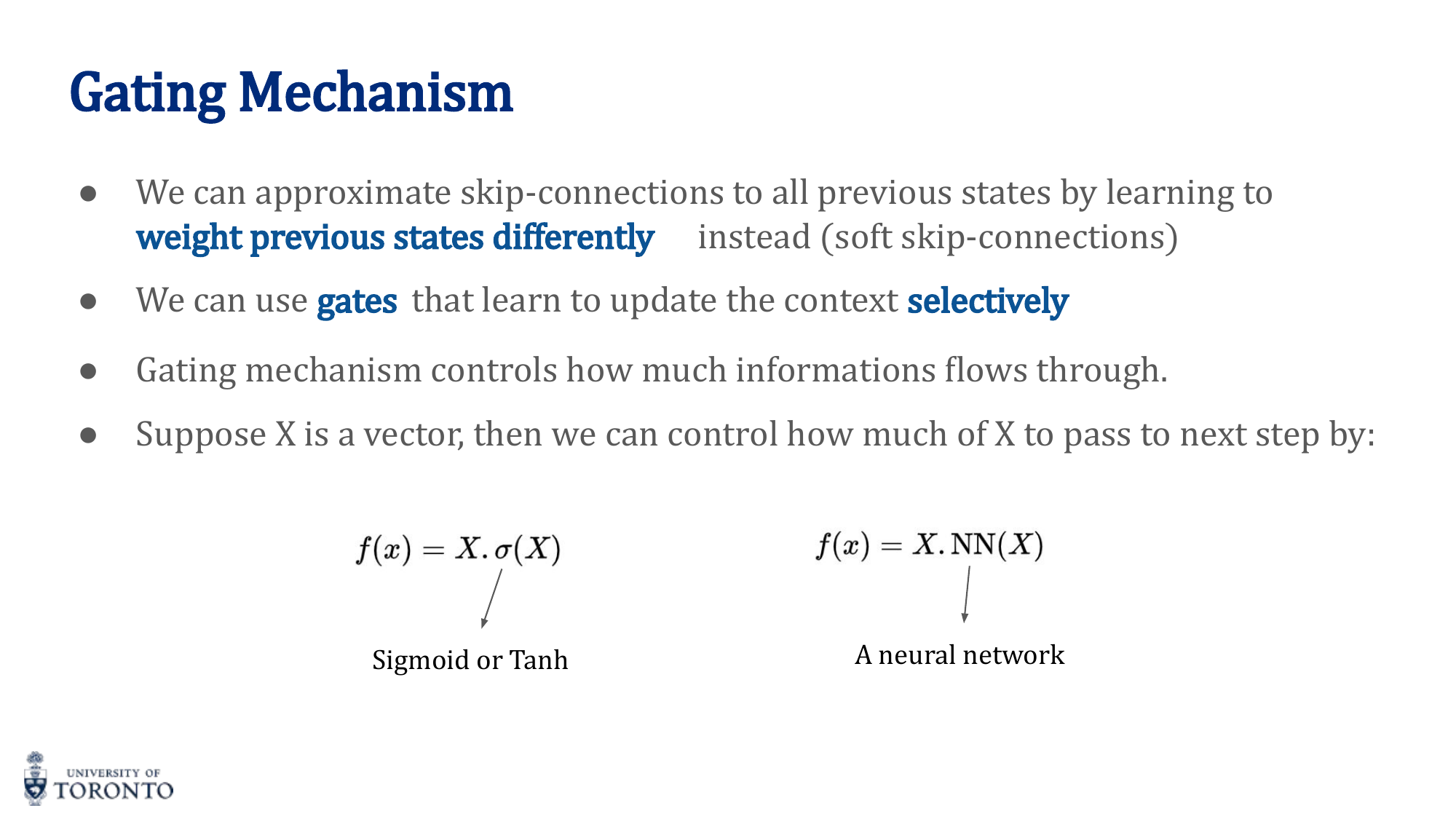
- Gating mechanisms (for vanishing): LSTM, GRU — additive updates instead of multiplicative
- Skip connections: Allow gradients to flow directly across time steps
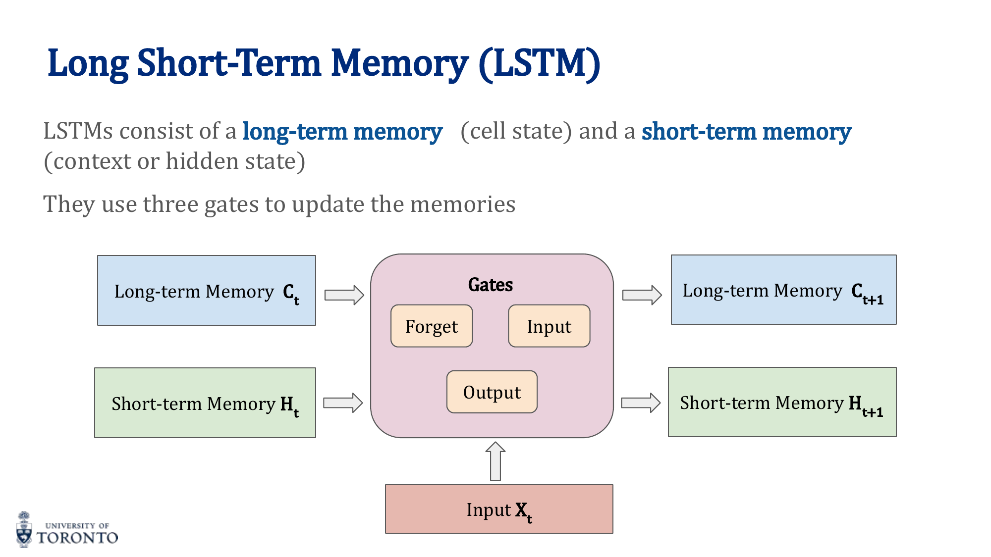
LSTM (Long Short-Term Memory)
LSTMs solve vanishing gradients by introducing a separate cell state (long-term memory) alongside the hidden state (short-term memory). Three gates control information flow:

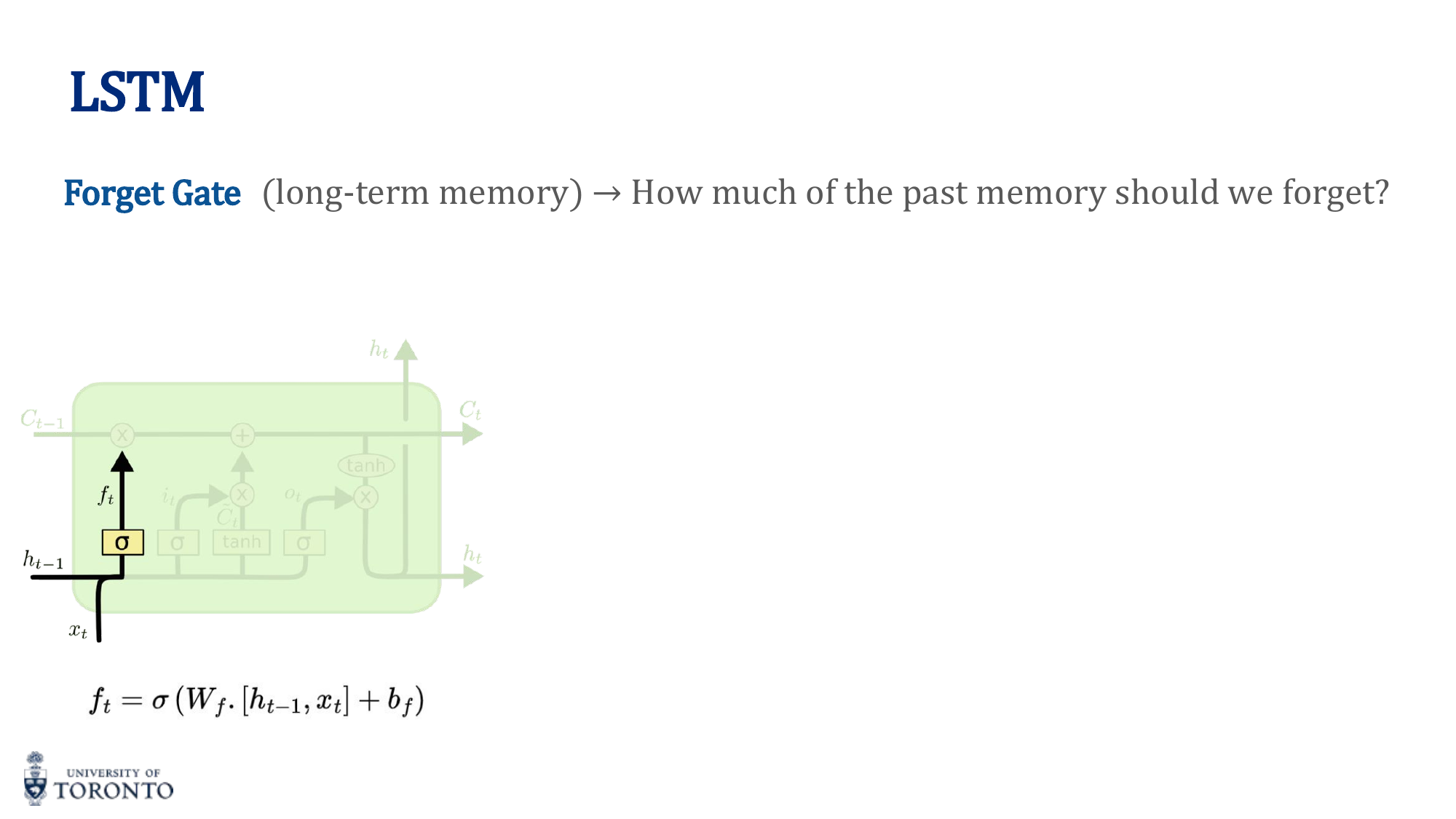
1. Forget Gate
Decides what to forget from the cell state:
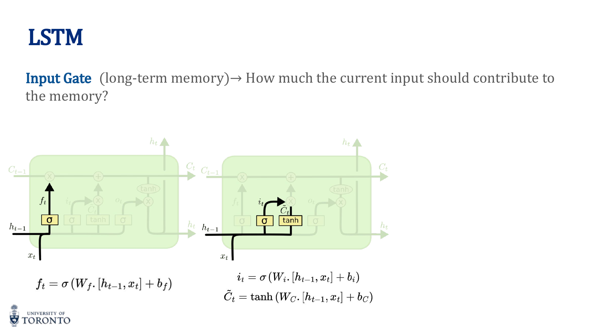
2. Input Gate
Decides what new information to add:
C̃_t = tanh(W_C · [h_(t-1), x_t] + b_C)
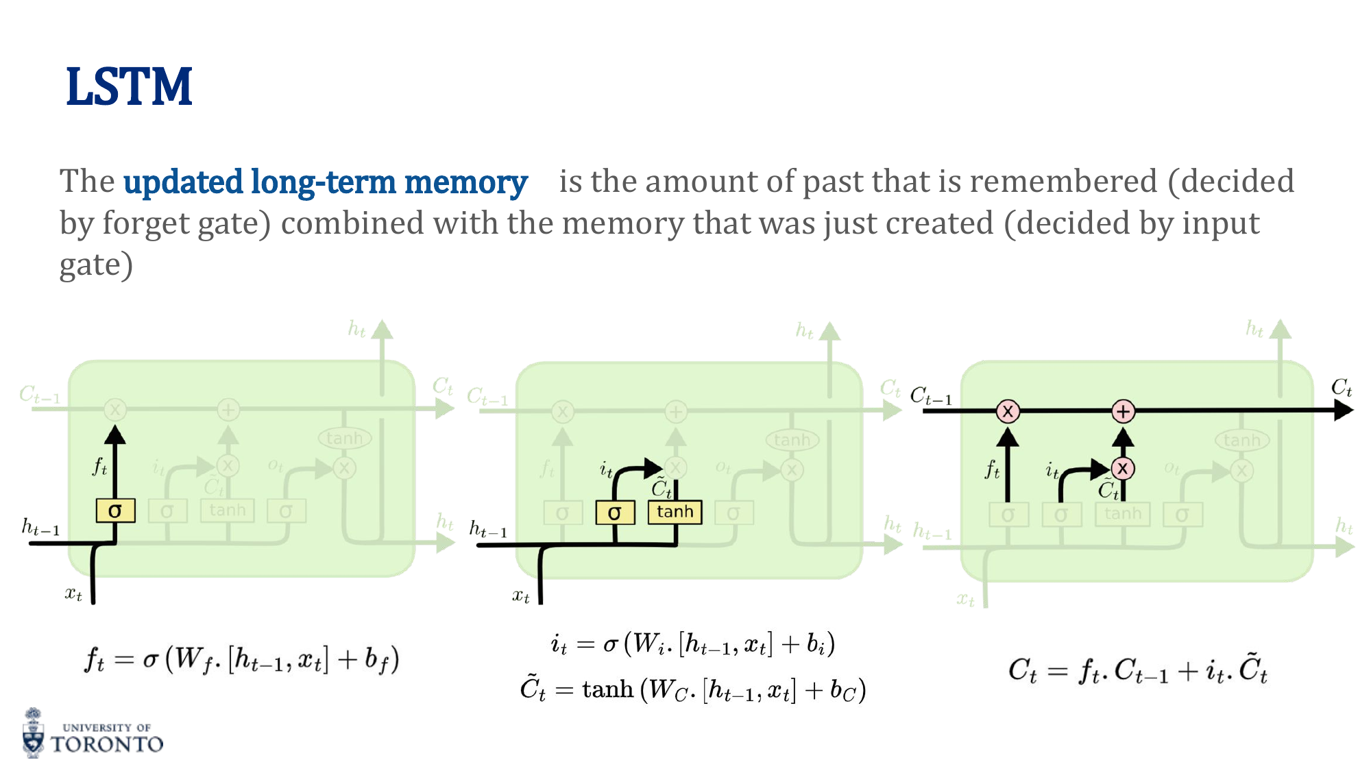
3. Cell State Update
Old cell state, selectively forgotten, plus new candidate values, selectively written.
4. Output Gate
Decides what to output as hidden state:
h_t = o_t · tanh(C_t)
Key Insight
Why LSTMs work: The cell state acts as a "conveyor belt" where information flows with only minor linear interactions (multiply by forget gate, add new info). Unlike the hidden state in vanilla RNNs (which undergoes matrix multiplication + nonlinearity at every step), the cell state update is additive. This makes it much easier for gradients to flow backward through many time steps without vanishing.
GRU (Gated Recurrent Unit)
A simplified version of LSTM with two gates (instead of three). Combines the forget and input gates into a single update gate, and merges cell state and hidden state:
| Property | LSTM | GRU |
|---|---|---|
| Gates | 3 (forget, input, output) | 2 (update, reset) |
| States | Cell state + hidden state | Hidden state only |
| Parameters | More (heavier) | Fewer (lighter) |
| Performance | Slightly better on long sequences | Comparable, trains faster |
# PyTorch: LSTM for sequence classification
class LSTMClassifier(nn.Module):
    def __init__(self, vocab_size, embed_dim, hidden_dim, num_classes):
        super().__init__()
        self.embedding = nn.Embedding(vocab_size, embed_dim)
        self.lstm = nn.LSTM(embed_dim, hidden_dim, batch_first=True)
        self.fc = nn.Linear(hidden_dim, num_classes)

    def forward(self, x):
        embedded = self.embedding(x)           # (B, T, embed_dim)
        output, (h_n, c_n) = self.lstm(embedded) # h_n: last hidden state
        logits = self.fc(h_n.squeeze(0))       # Use last hidden state
        return logits

# GRU: simply replace nn.LSTM with nn.GRU
# self.gru = nn.GRU(embed_dim, hidden_dim, batch_first=True)
# output, h_n = self.gru(embedded)  # No cell state returned
Section VIII
Generative Adversarial Networks
Week 9 • GANs, DCGAN & Adversarial Training
While discriminative models learn the boundary between classes (p(y|x)), generative models learn the underlying data distribution itself (p(x)). Generative Adversarial Networks frame this learning problem as a game between two competing networks: a generator that creates fake data and a discriminator that tries to distinguish real from fake.
Generative vs. Discriminative Models
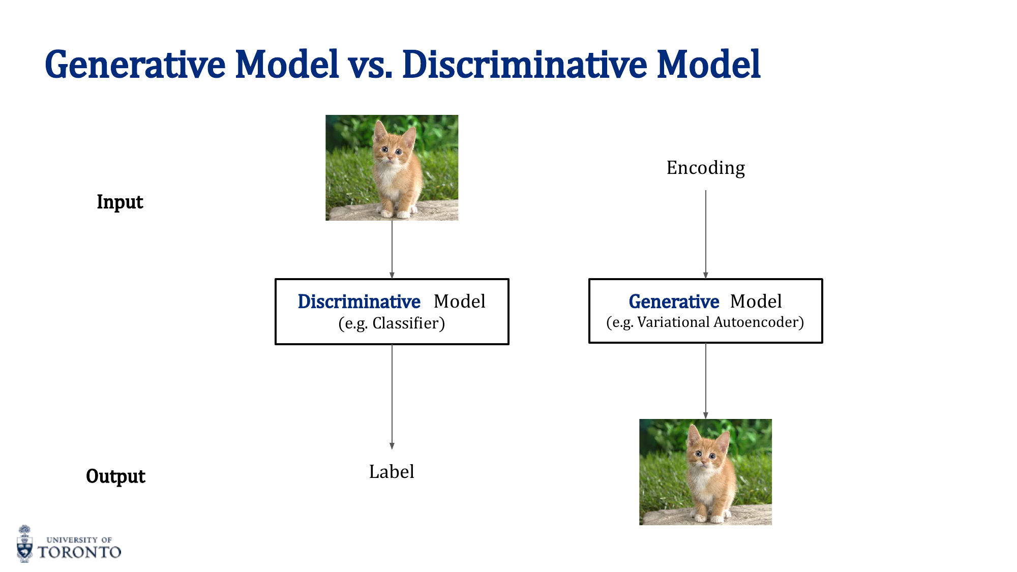
- Discriminative: Learns p(y|x) — "given this input, what's the label?" (classification, regression)
- Generative: Learns p(x) — "what does this type of data look like?" (generation, density estimation)
Families of Generative Models
- Autoregressive: Generate one element at a time, conditioned on previous elements
- VAEs: Probabilistic encoder-decoder with smooth latent space (covered in Week 6)
- GANs: Adversarial training between generator and discriminator (this lecture)
- Flow-based: Invertible transformations for exact likelihood computation
- Diffusion: Gradually denoise random noise into data
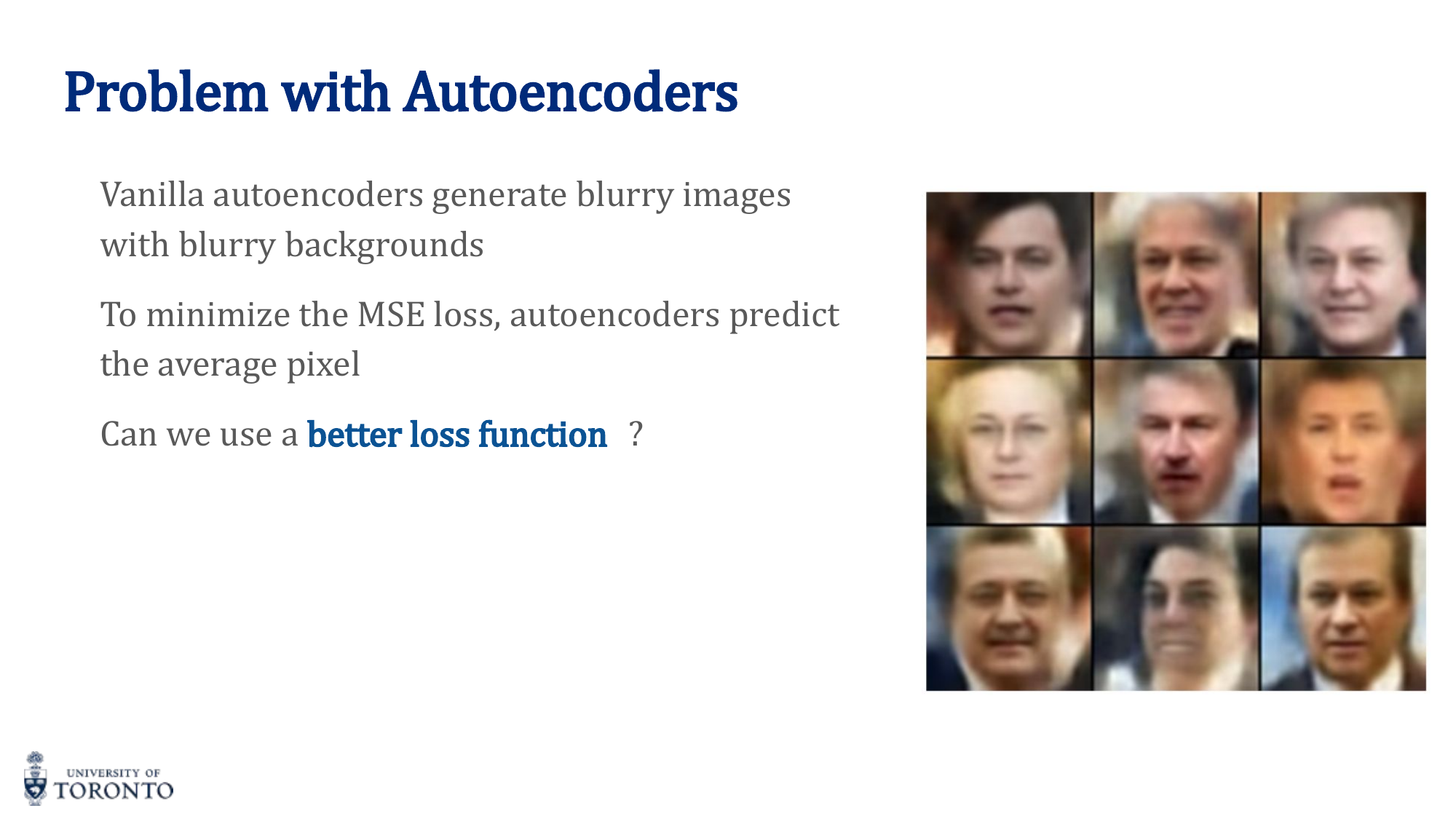
Why Not Just Autoencoders?
Autoencoders with MSE loss produce blurry images. MSE penalizes pixel-level differences, causing the model to predict the average pixel value (hedging its bets). GANs avoid this because the discriminator provides a more sophisticated, adversarial loss signal.
GAN Architecture
- Generator G: Takes random noise z ~ N(0,1) as input, outputs a fake image G(z)
- Discriminator D: Takes an image (real or fake) as input, outputs probability of being real D(x)
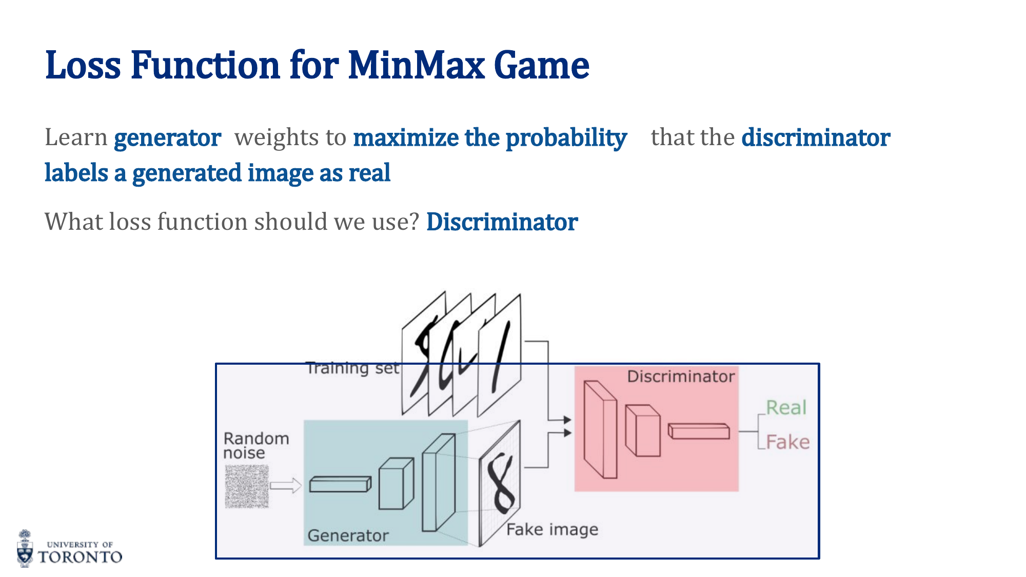
The MinMax Game
- D wants to maximize: D(real) → 1 and D(fake) → 0 (correct classification)
- G wants to minimize: D(G(z)) → 1 (fool the discriminator)
GAN Training Algorithm
- Train Discriminator: Sample real images and fake images (from G). Train D to classify them correctly using BCE loss.
- Train Generator: Generate fake images, pass through D. Train G to maximize D's probability of classifying fakes as real. Do NOT update D during this step.
- Alternate between steps 1 and 2.
Conditional vs. Unconditional
- Unconditional: Generator takes only noise — no control over what is generated
- Conditional: Generator receives noise + class label (one-hot) — can specify what to generate (e.g., "generate a 7")
Training Instabilities
- Mode collapse: Generator produces only a few types of outputs, ignoring the diversity of the data
- Non-convergence: G and D oscillate without reaching equilibrium
- Vanishing gradients for G: If D becomes too good, D(G(z)) ≈ 0 everywhere, giving G no gradient signal
DCGAN (Deep Convolutional GAN)
Uses convolutional layers for both G and D. Key design principles:
- Generator: Uses
ConvTranspose2d(transposed convolution / fractional strided convolution) for upsampling from noise to image - Discriminator: Uses
Conv2dfor downsampling from image to classification - Batch normalization in both networks
- ReLU in generator, LeakyReLU in discriminator
- No fully connected layers (except input/output)
Key Insight
GANs learn through competition. The generator never sees real data directly — it only receives gradient signals from the discriminator. As the discriminator gets better at detecting fakes, the generator must produce more realistic outputs to fool it. This adversarial dynamic pushes both networks to improve, but makes training inherently unstable compared to standard supervised learning.
# PyTorch: Simple GAN Training Loop
criterion = nn.BCELoss()
optim_D = torch.optim.Adam(D.parameters(), lr=2e-4, betas=(0.5, 0.999))
optim_G = torch.optim.Adam(G.parameters(), lr=2e-4, betas=(0.5, 0.999))

for epoch in range(num_epochs):
    for real_images, _ in dataloader:
        batch_size = real_images.size(0)
        real_labels = torch.ones(batch_size, 1)
        fake_labels = torch.zeros(batch_size, 1)

        # --- Train Discriminator ---
        z = torch.randn(batch_size, latent_dim)
        fake_images = G(z).detach()          # Don't update G here

        loss_D = criterion(D(real_images), real_labels) + \
                 criterion(D(fake_images), fake_labels)
        optim_D.zero_grad()
        loss_D.backward()
        optim_D.step()

        # --- Train Generator ---
        z = torch.randn(batch_size, latent_dim)
        fake_images = G(z)
        loss_G = criterion(D(fake_images), real_labels)  # Fool D
        optim_G.zero_grad()
        loss_G.backward()
        optim_G.step()
Section IX
Transformers
Week 10 • Attention, Self-Attention & the Transformer Architecture
Recurrent architectures process sequences one step at a time, creating an inherent bottleneck for parallelization and making it difficult to capture long-range dependencies. The Transformer architecture, introduced in "Attention Is All You Need" (2017), replaces recurrence entirely with attention mechanisms, enabling massive parallelization and direct connections between any two positions in a sequence.
RNN Limitations
- Sequential processing: Cannot parallelize — each step depends on the previous
- Long-range dependencies: Even LSTMs struggle with very long sequences
- Gradient issues: Vanishing/exploding gradients despite gating mechanisms
- Fixed-size hidden state: All sequence information must be compressed into one vector
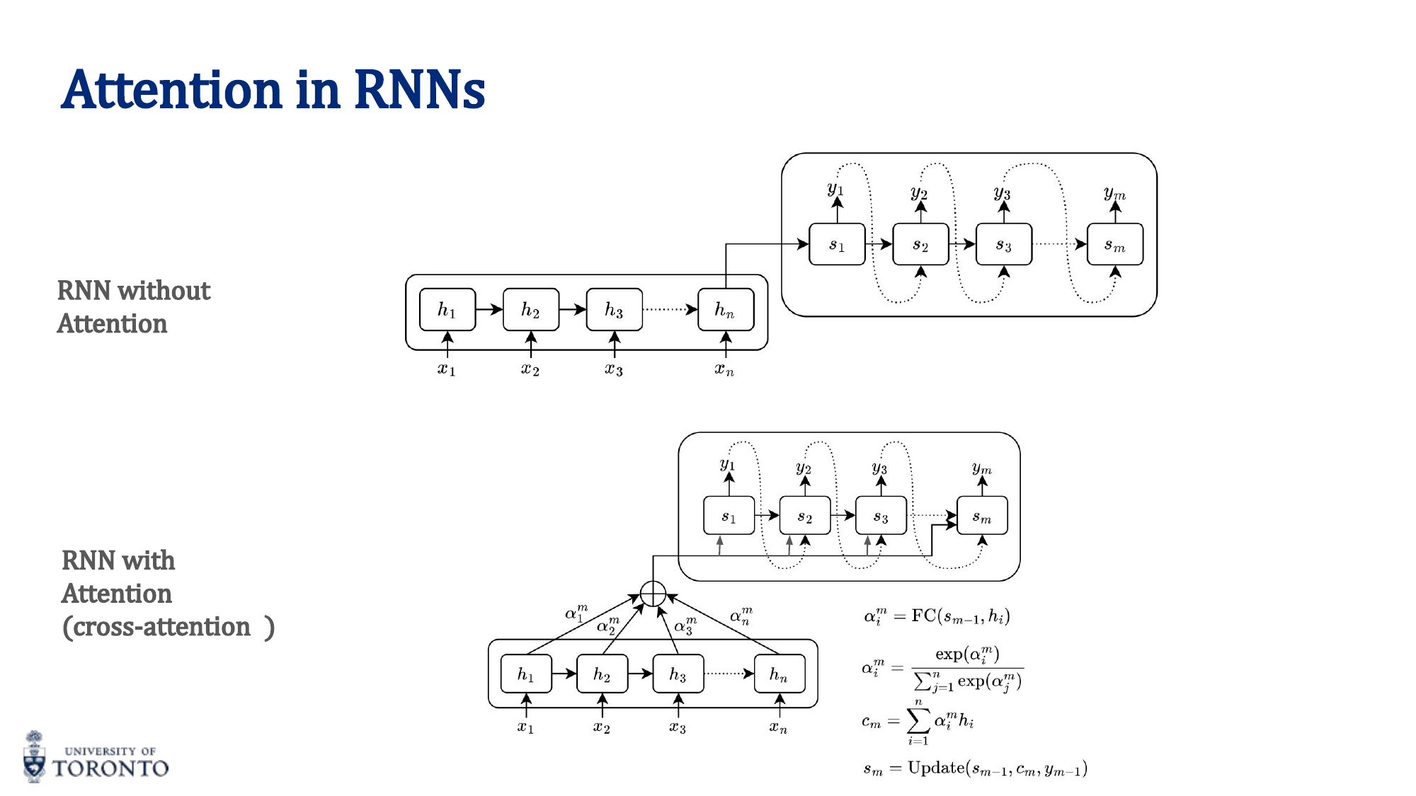
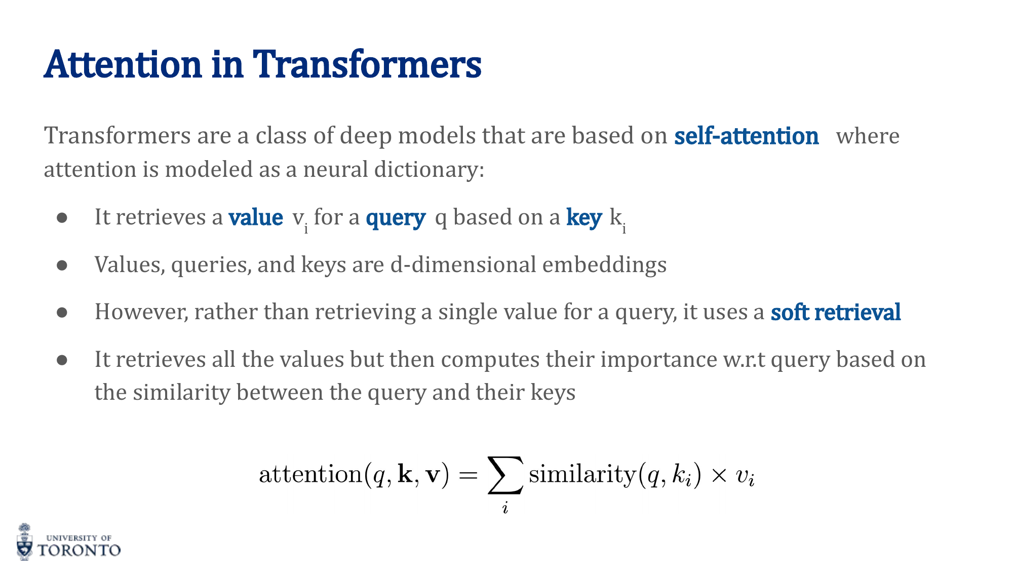
Attention Mechanism
Attention allows the model to focus on different parts of the input with different weights, rather than compressing everything into a single vector.
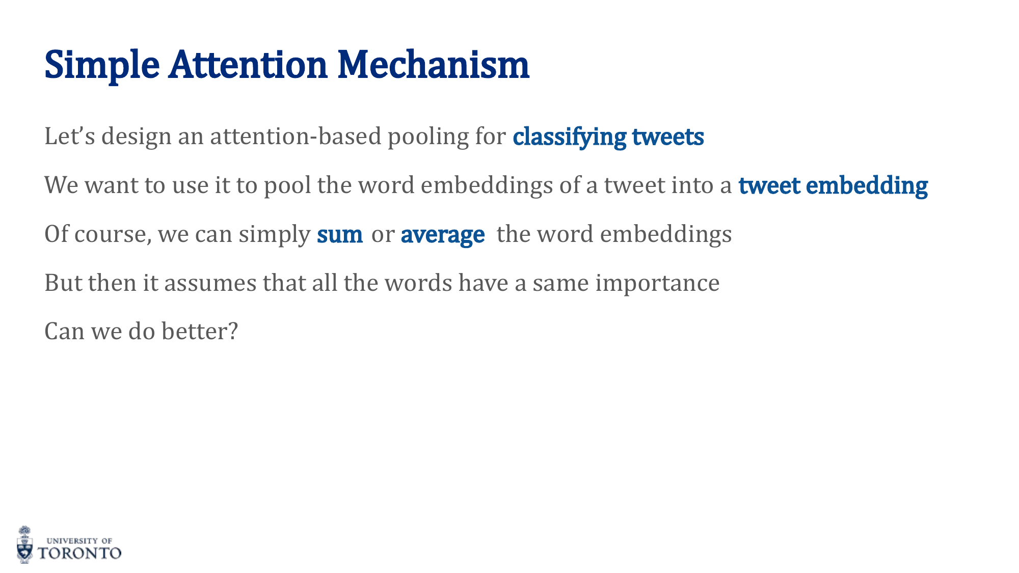
Simple Attention
For each position, compute a weighted sum of all positions' representations:
- Compute a score for each input position (via FC network, dot product, etc.)
- Normalize scores with softmax to get attention weights α
- Compute context vector: c_i = ∑ α_ij · h_j
Attention Score Methods
| Method | Formula |
|---|---|
| Dot product | score(a, b) = a^T b |
| Cosine similarity | score(a, b) = (a^T b) / (||a|| ||b||) |
| Bilinear | score(a, b) = a^T W b |
| MLP / Additive | score(a, b) = v^T tanh(W[a;b]) |
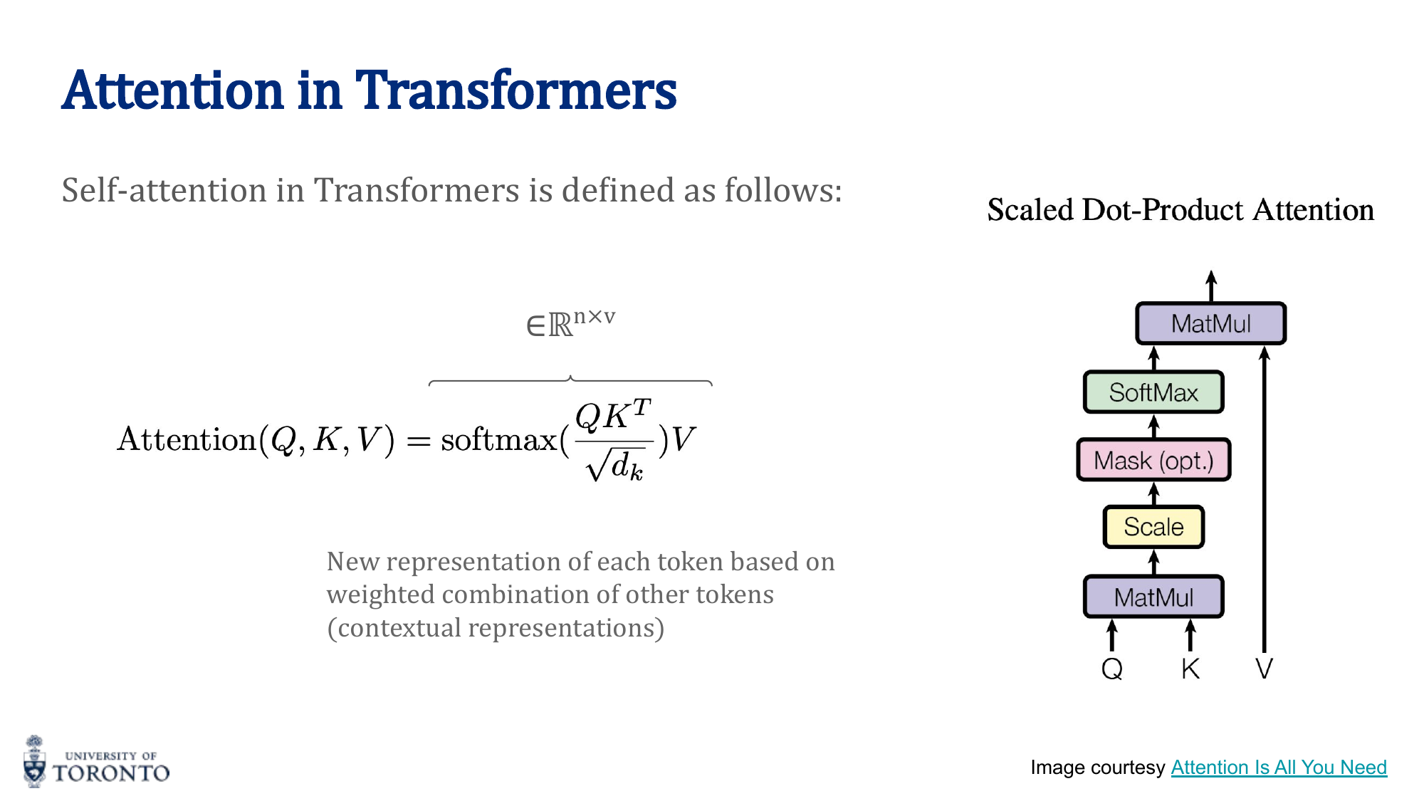
Self-Attention in Transformers
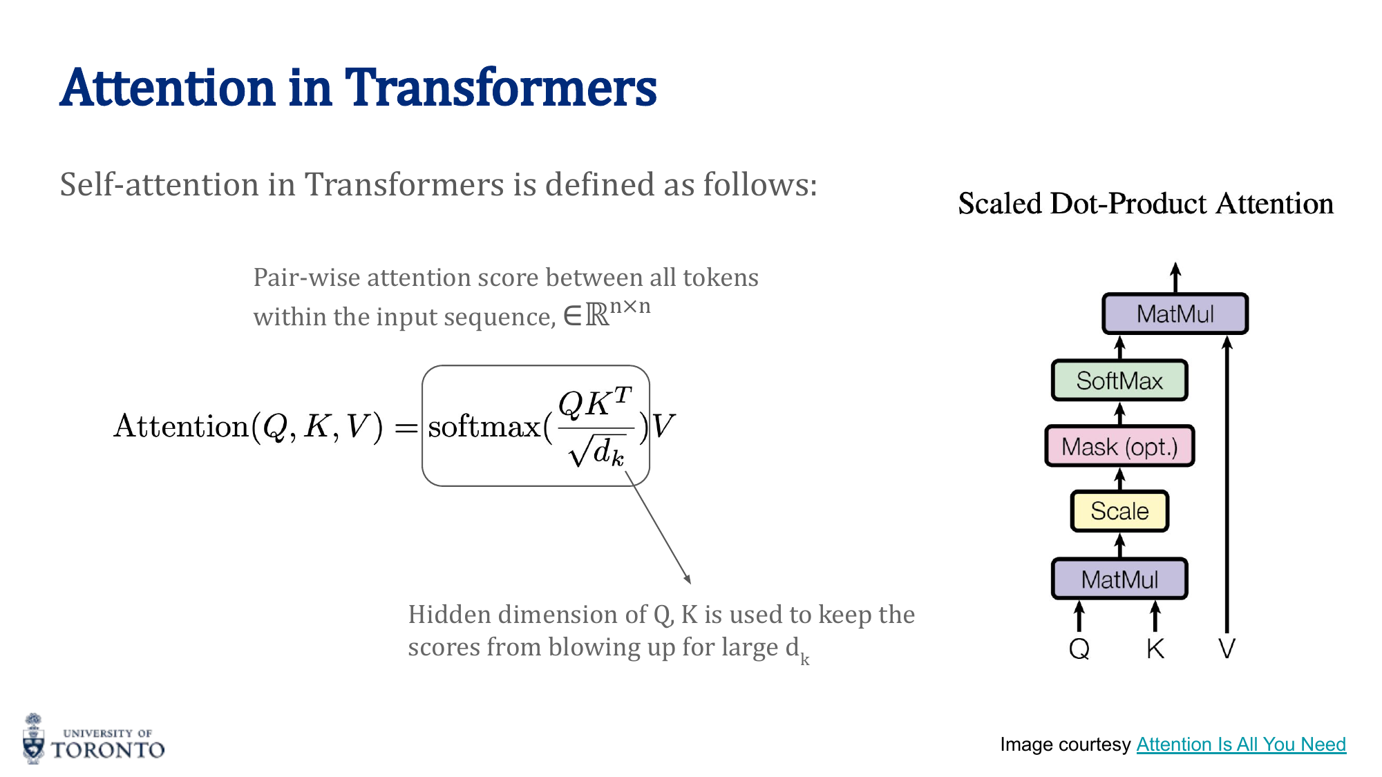
Self-attention computes attention between all positions within the same sequence. Each token looks at every other token (including itself) to gather context.
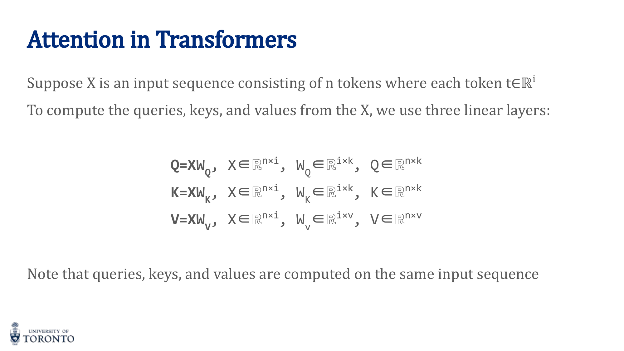
Three learned linear projections transform each input into:
- Query (Q): "What am I looking for?" — Q = X · W_Q
- Key (K): "What do I contain?" — K = X · W_K
- Value (V): "What information do I provide?" — V = X · W_V
Scaled Dot-Product Attention
The scale factor √d_k prevents the dot products from becoming too large (which would push softmax into saturated regions with near-zero gradients).
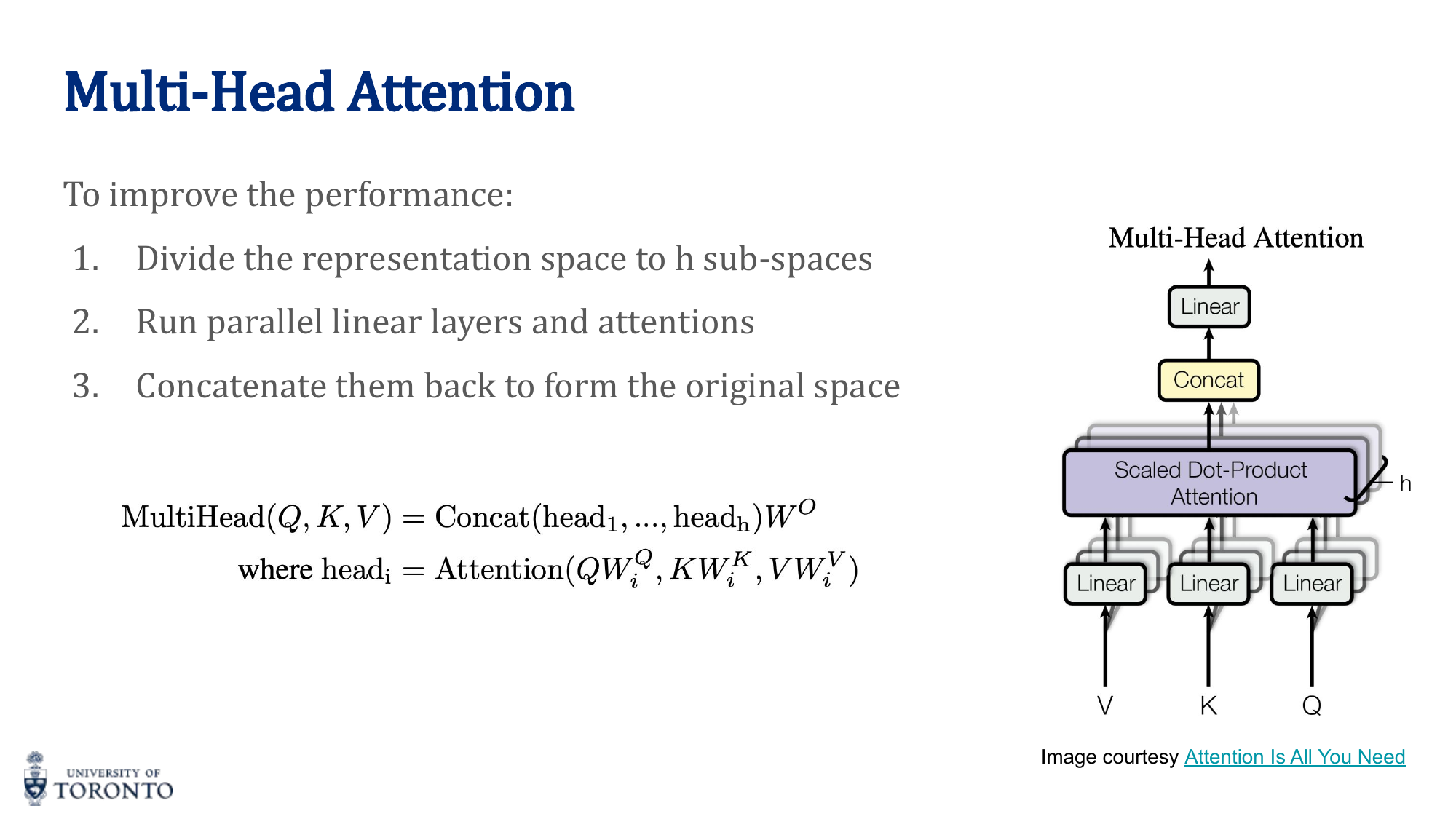
Multi-Head Attention
Instead of a single attention function, split Q, K, V into h parallel "heads." Each head learns different attention patterns (e.g., syntactic, semantic, positional):
where head_i = Attention(Q · W_Q^i, K · W_K^i, V · W_V^i)
Transformer Encoder Block
Each encoder block consists of:
- Multi-Head Self-Attention
- Add & Layer Normalization (residual connection)
- Position-wise Feed-Forward Network: FFN(x) = max(0, xW_1 + b_1)W_2 + b_2
- Add & Layer Normalization (residual connection)
This block is repeated N times (typically N=6 in the original Transformer).
Positional Encoding
Transformers have no recurrence, so they have no inherent notion of position. Positional encodings are added to the input embeddings:
PE(pos, 2i+1) = cos(pos / 10000^(2i/d))
Each position gets a unique encoding. The sinusoidal pattern allows the model to generalize to sequence lengths not seen during training.
Key Insight
RNN vs. Transformer: RNNs are O(n) sequential steps; information from position 1 must pass through every intermediate position to reach position n. Transformers connect every position to every other position directly in O(1), with O(n^2) total attention computations that can all happen in parallel. This makes Transformers dramatically faster to train and better at capturing long-range dependencies.
Transformer Variants
BERT (Bidirectional Encoder Representations from Transformers)
Encoder-only transformer. Pre-trained with Masked Language Modeling (randomly mask 15% of tokens, predict them). Bidirectional — attends to both left and right context. Fine-tuned for downstream NLP tasks (classification, NER, QA).
GPT (Generative Pre-trained Transformer)
Decoder-only transformer. Uses masked (causal) self-attention — each position can only attend to earlier positions (autoregressive generation). Pre-trained with next-token prediction. Generates text left-to-right.
Vision Transformer (ViT)
Applies the transformer to images: split the image into fixed-size patches (e.g., 16×16), flatten each patch, linearly project, add positional encoding, and process as a sequence of tokens with a standard transformer encoder.
# PyTorch: Transformer Encoder
encoder_layer = nn.TransformerEncoderLayer(
    d_model=512,    # Embedding dimension
    nhead=8,        # Number of attention heads
    dim_feedforward=2048,
    dropout=0.1
)
transformer_encoder = nn.TransformerEncoder(encoder_layer, num_layers=6)

# Self-attention from scratch
def scaled_dot_product_attention(Q, K, V):
    d_k = Q.size(-1)
    scores = torch.matmul(Q, K.transpose(-2, -1)) / (d_k ** 0.5)
    weights = torch.softmax(scores, dim=-1)
    return torch.matmul(weights, V)
Section X
Graph Neural Networks
Week 11 • Message Passing, GCN & GAT
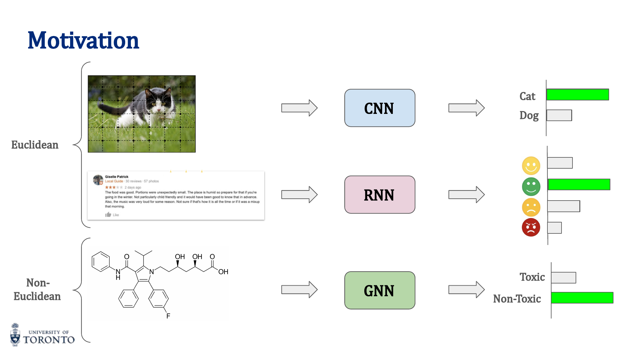
CNNs excel on grid-structured data (images) and RNNs on sequential data (text), but many real-world problems have non-Euclidean structure: molecular graphs, social networks, 3D meshes, knowledge graphs. Graph Neural Networks extend deep learning to arbitrary graph structures, learning representations that respect the topology of the data.
Motivation
Graph Definitions
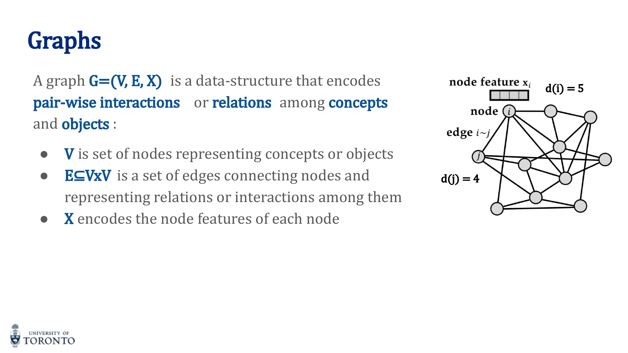
A graph G = (V, E, X) consists of:
- V: Set of nodes (vertices)
- E ⊆ V × V: Set of edges connecting nodes
- X: Node feature matrix (each node has a feature vector)
Adjacency Matrix
A square matrix A where a_ij = 1 if there is an edge between nodes i and j, 0 otherwise. For undirected graphs, A is symmetric.
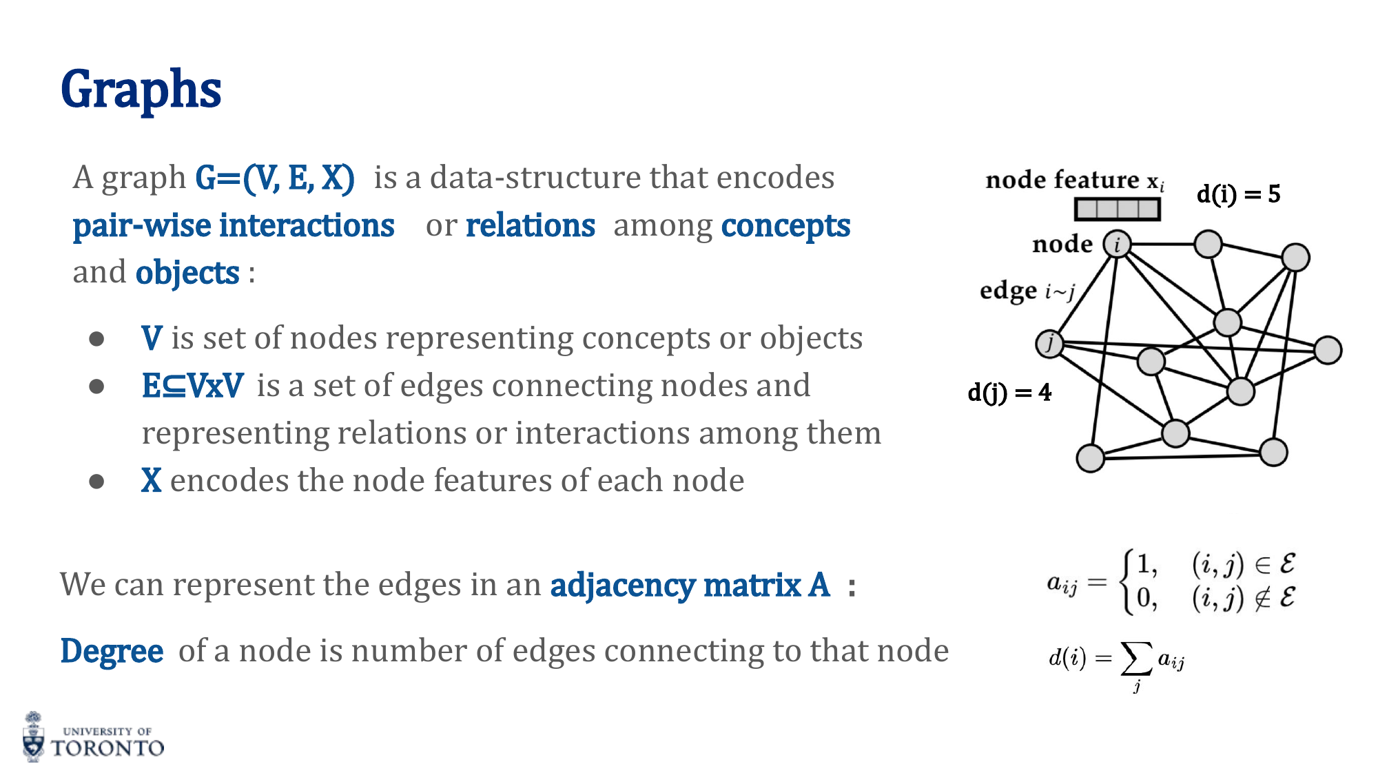
Degree
The degree d(i) of a node is the number of edges connected to it: d(i) = ∑_j a_ij
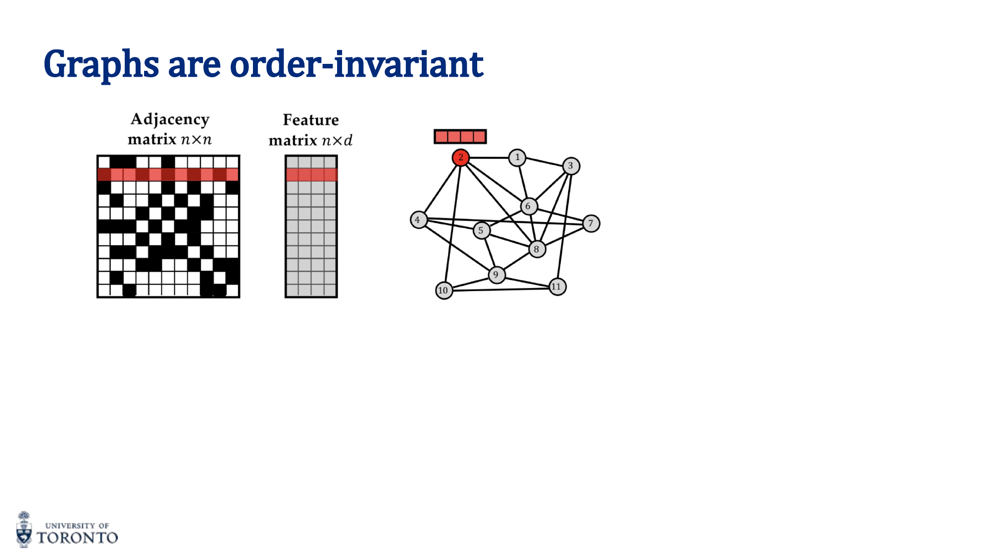
Order Invariance
Graphs are order-invariant: the same graph can be represented with n! different node orderings. A valid GNN must produce the same output regardless of how nodes are numbered.
Key Insight
Transformers and Graphs: A transformer without positional encoding is equivalent to a fully-connected graph where every node attends to every other node with learned edge weights (attention scores). Graphs generalize this: instead of full connectivity, only neighboring nodes exchange information.
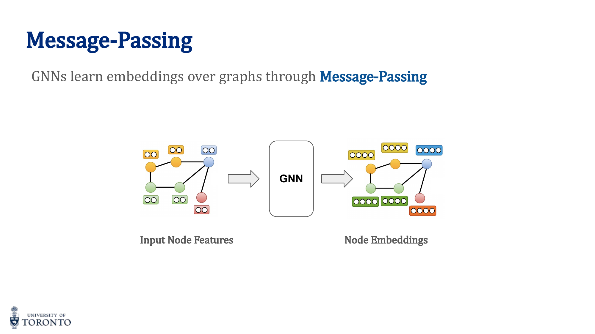
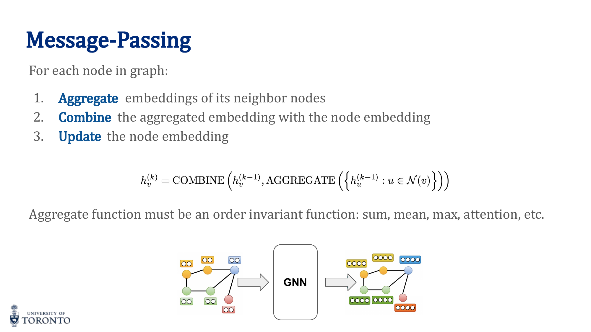
Message Passing
The core operation in GNNs. For each node, at each layer:
- Aggregate: Collect embeddings from all neighbor nodes
- Combine: Merge aggregated neighbor information with the node's own embedding
- Update: Apply a transformation (e.g., linear layer + activation)
Aggregation functions must be order-invariant (permutation invariant):
- Sum: Captures total neighborhood information (sensitive to degree)
- Mean: Captures average neighborhood information (degree-normalized)
- Max: Captures the most prominent feature across neighbors
- Attention: Weighted sum with learned attention weights (GAT)
GNN Tasks
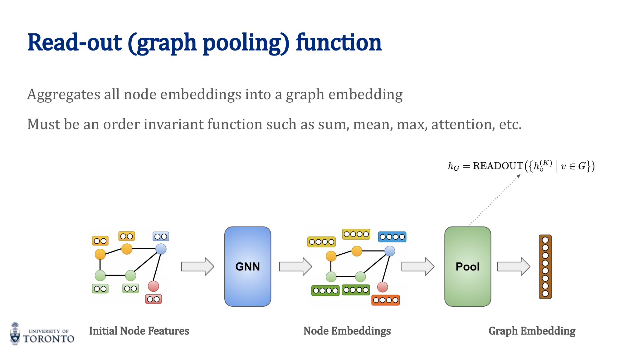
Graph-Level Readout (Pooling)
For graph-level tasks, aggregate all node embeddings into a single graph embedding:
Common readout functions: sum, mean, max over all node embeddings.
Graph Convolutional Networks (GCN)
The simplest GNN. Each layer computes:
Limitations of naive GCN:
- Does not include self-features (node doesn't aggregate from itself) — fix: use A + I (add self-loops)
- Nodes with different degrees get embeddings at different scales — fix: normalize by degree
Normalized GCN
Where  = A + I (adjacency with self-loops) and D̂ is the degree matrix of Â. The symmetric normalization ensures consistent scaling regardless of node degree.
Graph Attention Networks (GAT)
Instead of treating all neighbors equally (GCN) or using simple mean/sum aggregation, GAT uses attention to learn different importance weights for different neighbors:
- Compute attention coefficients between connected nodes
- Normalize with softmax over the neighborhood
- Weighted aggregation based on learned attention weights
- Can use multi-head attention (like transformers)
# PyTorch Geometric: GCN
from torch_geometric.nn import GCNConv

class GCN(nn.Module):
    def __init__(self, in_features, hidden_dim, num_classes):
        super().__init__()
        self.conv1 = GCNConv(in_features, hidden_dim)
        self.conv2 = GCNConv(hidden_dim, num_classes)

    def forward(self, x, edge_index):
        x = self.conv1(x, edge_index)
        x = torch.relu(x)
        x = self.conv2(x, edge_index)
        return x

# For graph classification, add global pooling:
# from torch_geometric.nn import global_mean_pool
# graph_embedding = global_mean_pool(x, batch)
# output = self.classifier(graph_embedding)
Based on Past Final Exams • Winter & Summer 2025
Final Exam Focus
This section distills the lecture content most critical for the final exam, based on analysis of past papers. Topics are ranked by how frequently and heavily they are tested. Each section teaches the theory, key equations, and computational techniques you need to solve any exam question on that topic.
Focus Area 1 • Highest Priority
Recurrent Neural Networks, LSTMs & GRUs
Tested Every Exam • 20–30+ Marks Combined
Vanilla RNN Recurrence
The hidden state at time t is computed from the previous hidden state and the current input:
where xt ∈ ℝd is the input, ht ∈ ℝH is the hidden state, and bh ∈ ℝH is the bias.
Critical Dimensions — Exam Favourite
Whh ∈ ℝH×H (maps hidden-to-hidden)
Wxh ∈ ℝH×d (maps input-to-hidden)
bh ∈ ℝH
How ht is formed: The weighted sum of the previous hidden state ht-1 and the current input xt, plus bias, is passed through the tanh nonlinearity.
The Vanishing Gradient Problem
During backpropagation through time (BPTT), gradients are propagated through many time steps. Because the chain rule multiplies partial derivatives at each step, if the weight values lead to derivatives consistently less than 1, gradients shrink exponentially — they vanish. If greater than 1, they explode.
This makes it nearly impossible for vanilla RNNs to learn long-term dependencies in sequences. The error signal from distant time steps cannot effectively reach early layers.
Exam Tip
Vanishing gradients is the #1 tested concept for RNNs. Know that it happens because of repeated multiplication of small derivatives through tanh across time steps, and that LSTM/GRU solve it via gating mechanisms. Gradient clipping addresses exploding gradients.
Teacher Forcing
During training, instead of feeding the RNN’s own previous prediction as the next input, teacher forcing feeds the ground-truth token at each time step.
Benefit: It stabilizes and accelerates convergence by preventing the model from compounding its own errors early in training. Without it, one wrong prediction cascades into increasingly wrong subsequent predictions.
LSTM — Long Short-Term Memory
LSTMs solve the vanishing gradient problem by introducing a cell state ct that flows through time with additive updates (not multiplicative), and three gates that control information flow:
Input gate: it = σ(Wi xt + Ui ht-1 + bi)
Candidate: c̃t = tanh(Wc xt + Uc ht-1 + bc)
Cell update: ct = ft ⊙ ct-1 + it ⊙ c̃t
Output gate: ot = σ(Wo xt + Uo ht-1 + bo)
Hidden state: ht = ot ⊙ tanh(ct)
LSTM Dimensions — Know These Cold
Given xt ∈ ℝd and ht, ct ∈ ℝH:
Wf, Wi, Wc, Wo ∈ ℝH×d (input weight matrices)
Uf, Ui, Uc, Uo ∈ ℝH×H (recurrent weight matrices)
bf, bi, bc, bo ∈ ℝH (bias vectors)
Understanding Each Gate
- Forget gate (ft): Outputs values in [0,1]H. Scales each component of the previous cell state ct-1, deciding what to erase. A value of 0 = completely forget, 1 = fully retain.
- Input gate (it): Outputs values in [0,1]H. Scales the candidate c̃t, deciding what new information to add.
- Cell update: ct = ft ⊙ ct-1 + it ⊙ c̃t. This is why LSTMs preserve information — the additive structure allows gradients to flow without vanishing.
- Output gate (ot): Controls what portion of the cell state is exposed as the hidden state output.
Cell State vs. Hidden State
- Cell state ct: The “long-term memory.” Updated linearly (additive), so information can persist across many time steps without degradation.
- Hidden state ht: The “working memory” exposed at each time step. Computed by filtering ct through the output gate and tanh. This is what gets passed to the next layer or used for predictions.
- Why both? The cell state stores information broadly; the hidden state controls what to reveal. This separation gives the LSTM precise control over what is remembered vs. what is communicated.
GRU — Gated Recurrent Unit
Compared to LSTM, a GRU has fewer gates and fewer parameters. It merges the cell state and hidden state into a single state, and uses only two gates (reset and update) instead of three. This makes GRUs faster to train while achieving similar performance on many tasks.
Exam Favourite MC Question
“Compared to an LSTM, a GRU typically has:” → Fewer gates and fewer parameters (Answer C). This is tested almost every exam.
Focus Area 2 • Highest Priority
Graph Neural Networks & GCNs
Tested Every Exam • 15–20+ Marks Combined
Message Passing Framework
GNNs operate on graph-structured data through message passing, which consists of three operations at each layer:
- Message: Each node sends a message (typically its current embedding) to its neighbours.
- Aggregate: Each node collects messages from all its neighbours using a permutation-invariant function (e.g., sum, mean, max).
- Update: Each node combines the aggregated message with its own previous embedding to form a new embedding.
Exam Distinction — Aggregate vs. Update
Aggregate = collecting messages from all neighbours.
Update = combining the aggregated message with the node’s own previous embedding.
These are different steps — the exam tests whether you can distinguish them.
Permutation Invariance
Graphs have no inherent ordering of nodes. If you relabel or reorder the neighbours of a node, the aggregated result must remain the same. This is why the aggregation function must be permutation invariant.
Functions like sum, mean, and max are permutation invariant. Concatenation is not, because order matters.
MC Favourite
The aggregation function must be “permutation invariant and often realized through commutative and associative operations.” This exact phrasing appears in past exams.
The GCN Layer Equation
A single Graph Convolutional Network layer is defined by:
where:
- A ∈ {0,1}N×N — adjacency matrix of the undirected graph
- Â = A + IN — adjacency with self-loops added
- D̂ — diagonal degree matrix of Â
- H(l) ∈ ℝN×F — node embeddings at layer l (N nodes, F features)
- W(l) ∈ ℝF×F′ — learnable weight matrix
- σ — element-wise nonlinearity (e.g., ReLU)
Key Dimensions — Always Tested
 ∈ ℝN×N
D̂-1/2 ∈ ℝN×N
H(l+1) ∈ ℝN×F′
Why Self-Loops (A + IN)?
Using A directly means a node aggregates only its neighbours’ features, not its own. Adding the identity matrix IN creates self-loops, ensuring each node’s own features are included in its update. Without this, a node’s identity would be lost after aggregation.
Why Normalization (D̂-1/2)?
The adjacency matrix is not normalized, so multiplying by it can change the scale of node features — especially for high-degree nodes. The symmetric normalization D̂-1/2 Â D̂-1/2 normalizes each entry by the geometric mean of the degrees, preventing scale explosion.
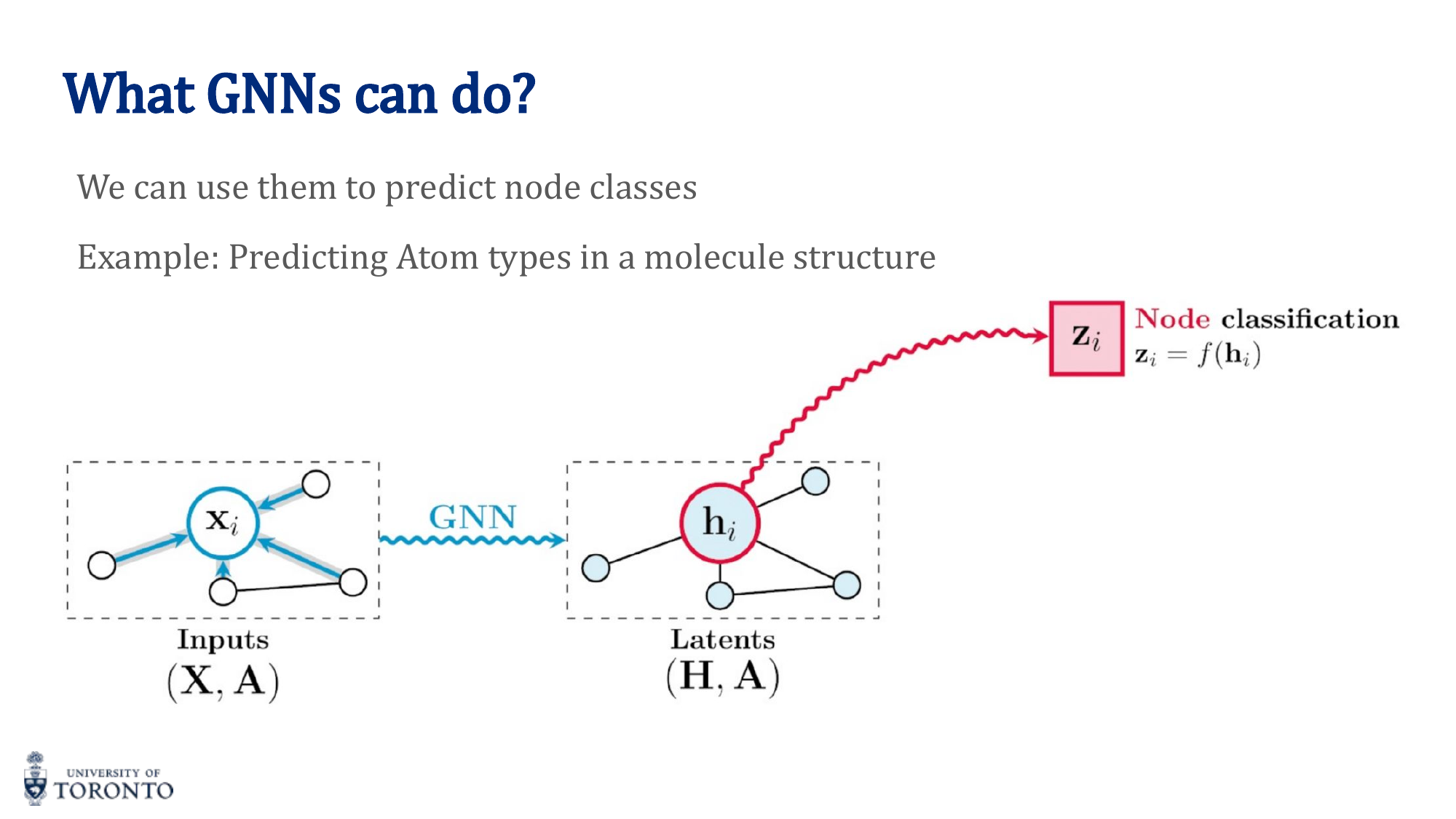
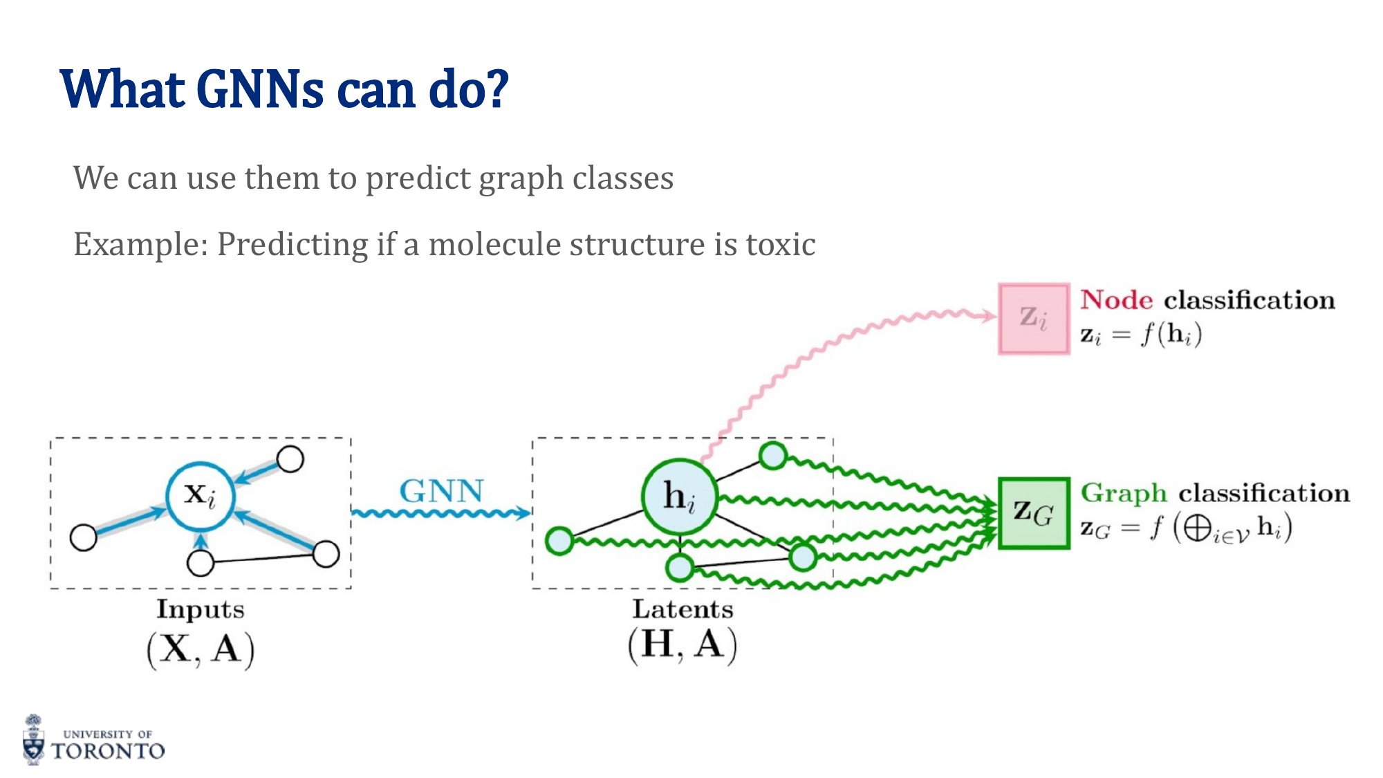
Node vs. Graph Classification
- Node classification: Assigns labels to individual nodes (not entire graphs, edges, or substructures).
- Graph classification: Requires a readout/pooling step to produce a single graph-level embedding from all node embeddings.
Readout Functions
To produce a graph-level embedding from node embeddings, use a permutation-invariant readout:
- Global sum pooling
- Global mean pooling
- Global max pooling
- Attention readout
Why permutation invariant? Nodes in a graph have no natural order. The graph embedding must be the same regardless of how you index or iterate over the nodes.
Sum vs. Attention-Based Aggregation
Sum aggregation: Each neighbour’s embedding is weighted equally. Simple and efficient, but cannot capture the varying importance of different neighbours.
Attention-based aggregation (GAT): Learns a weight (attention score) for each neighbour, allowing the model to focus more on important neighbours and less on irrelevant ones. More expressive but more parameters.
Focus Area 3 • High Priority
Generative Adversarial Networks
Tested Every Exam • 10–15+ Marks
Generator & Discriminator
A GAN consists of two networks trained in an adversarial game:
- Generator G(z): Maps random noise z to synthetic samples. Goal: fool the discriminator into classifying fake samples as real.
- Discriminator D(x): Distinguishes real data x from fake samples G(z). Goal: correctly classify real vs. fake.
- Adversarial interaction: The generator improves to fool the discriminator; the discriminator improves to detect the generator. They push each other to improve.
Loss Functions
- Discriminator loss: Binary Cross-Entropy (BCE) — maximize probability of correctly labelling real as real and fake as fake.
- Generator loss: Minimize the discriminator’s ability to correctly classify — effectively, maximize D(G(z)). The generator’s loss is the discriminator’s loss on fake samples.
Mode Collapse
Mode collapse occurs when the generator produces images for only a few classes or modes of the data distribution, ignoring the full diversity. This happens because the discriminator gets trapped in a local minimum and cannot distinguish fake from real in those specific classes, so the generator exploits this weakness rather than learning the full distribution.
CycleGAN
CycleGAN performs unpaired image-to-image translation (e.g., horse ↔ zebra). It consists of:
- Main generator: Generates images with correct objects and postures.
- Discriminator: Ensures the generated objects are correct (e.g., look like horses).
- Second generator (decoder): Ensures postures and geometry are preserved by reconstructing the original image.
Inputs and outputs of both generators are images. The discriminator outputs a binary label (real/fake).
Key Exam Points About CycleGAN
• The model is trained in a multi-task manner (GAN loss + reconstruction/cycle-consistency loss).
• All components are needed during training, but only the main generator is needed for inference.
• This is the correct MC answer: “The model is trained in a multi-task manner.”
Text-to-Image GANs
To design a GAN that takes a text description and generates an image:
- Introduce an RNN or Transformer encoder to encode the text into a conditioning vector.
- The text encoder is shared between generator and discriminator.
- Training data must be pairs of (text, image).
- Noise is not needed — the text provides the conditioning signal.
- Use transfer learning (e.g., pretrained BERT) for the text encoder to train faster with less data.
Focus Area 4 • High Priority
Variational Autoencoders
Tested Every Exam • 8–10+ Marks
VAE vs. Vanilla Autoencoder
A vanilla autoencoder maps each input to a single deterministic point in latent space (z = f(x)). A VAE instead learns a distribution over latent codes — the encoder outputs mean μ and variance σ², and we sample z from this distribution. This is what distinguishes a VAE from a vanilla AE.
Encoder Outputs
The encoder network outputs two vectors:
- μφ(x) ∈ ℝL — the mean of the approximate posterior qφ(z | x).
- σ²φ(x) ∈ ℝL — the variance, controlling the spread in each latent dimension.
Together they parameterize: qφ(z | x) = N(z; μφ, diag(σ²φ))
The VAE Loss Function
The training objective has two terms:
- Reconstruction loss: Measures how well the decoder can reconstruct the input from latent samples. Encourages accurate reconstruction.
- KL divergence term: Regularizes the learned latent distribution qφ(z|x) to stay close to the prior p(z) = N(0, I). Ensures the latent space is structured and allows meaningful sampling.
What If KL Is Omitted?
Without the KL divergence term, the encoder could overfit by assigning disjoint latent codes to each training example. The latent space would have “holes” — sampling from those holes would produce incoherent outputs. The KL term ensures smooth, continuous latent space.
Generating New Samples
Once trained, generation is a two-step process:
- Sample z ~ p(z) = N(0, I) from the prior in latent space.
- Decode by passing z through the trained decoder pθ(x | z) to obtain a new synthetic data point x.
Decoder Computation — Worked Example
Given a latent sample z, the decoder computes logits a = Wz + b, then applies activation g to get output x̂ = g(a). If g is linear, x̂ = a directly.
Exam Computation Pattern
You will be given W, b, and z. Compute a = Wz + b via matrix multiplication, then apply the activation. Practice this with 2×2 matrices — it always appears on the exam.
Focus Area 5 • High Priority
Transformers & Self-Attention
Tested Every Exam • 10–15+ Marks
Self-Attention Mechanism
Each input token begins as a static embedding. Self-attention transforms these into contextual embeddings by allowing each token to attend to all other tokens in the sequence:
- Static embeddings represent each word in isolation.
- Self-attention computes Query (Q), Key (K), and Value (V) matrices from the embeddings.
- Attention scores are computed as Q ⋅ KT, scaled by √dk, then softmax-normalized row-wise.
- The output is the weighted combination of V, where weights are the attention scores.
Incorrect Statement — Common MC Trap
“Multi-head attention assumes an undirected graph over the input sequence” is INCORRECT. It actually assumes a fully-connected graph (every token attends to every other token). Attention is directional — it can be masked (as in GPT) to be unidirectional.
Multi-Head Attention
With K heads, each head computes its own Q, K, V projections and its own attention matrix. The outputs are concatenated and linearly projected. With K heads, there are K separate attention matrices.
Positional Encoding
Transformers process all tokens in parallel and do not naturally encode order. Without positional encoding, the model would treat the sequence as a bag of words.
Positional encoding injects information about word order into the embeddings. By combining positional signals with attention, the model produces contextual embeddings that are sensitive to both content and order.
Dimension of Positional Encoding
The positional encoding has the same dimension as the feature/embedding dimension (so it can be added element-wise to the token embeddings). If feature dimension is 16, positional encoding dimension is 16.
Tensor Dimensions — Computation Questions
Given batch size B, sequence length L, feature dimension d, key/query dimension dk, value dimension dv, and H heads:
- Attention tensor (before head concatenation): B × H × L × L (each head has an L×L attention matrix)
- Output tensor (single head): B × L × dv
- Q, K projections: d × dk + dk (weights + biases) each
- V projection: d × dv + dv (weights + biases)
Parameter Counting in a Transformer Layer
A single transformer layer has attention projections + feed-forward network. For feature dim d, key dim dk, value dim dv, H heads, and FFN widths n1, n2:
V projection: d × dv + dv
FC layer 1: dv × n1 + n1
FC layer 2: n1 × n2 + n2
Total: H × (Q + K params) + V params + FC1 + FC2
Exam Pattern
You will be given specific numbers (e.g., d=16, dk=32, dv=64, H=2, FFN widths 100 and 200). You need to compute total parameters step by step. Don’t forget biases. Remember that Q and K parameters are multiplied by H (one per head), but V is shared.
Focus Area 6 • High Priority
Convolutional Neural Networks
Tested Every Exam • 10+ Marks
Conv Layers vs. Fully Connected Layers
Convolutional layers use local receptive fields and shared filters across spatial positions. This greatly reduces the number of parameters compared to fully connected layers, and captures spatially local patterns (edges, textures, shapes) — making CNNs especially effective for image data.
Parameter Counting — The Most Tested Skill
For a convolutional layer with Cin input channels, Cout filters, and kernel size k × k:
Worked Example — RGB Image with Two Conv Layers
Conv1: 3 input channels (RGB), 10 filters, 3×3 kernel → 3 × 10 × 3 × 3 + 10 = 280
Conv2: 10 input channels, 20 filters, 3×3 kernel → 10 × 20 × 3 × 3 + 20 = 1,820
Special Case: 1×1 Convolution
A conv layer that maps input of depth Cin to depth Cout with 1×1 kernel has: Cin × Cout × 1 × 1 + Cout parameters. For example, mapping depth 16 to depth 1: 16 × 1 + 1 = 17.
Output Size Formula
where n = input size, f = filter size, p = padding, s = stride.
Pooling Layers
Pooling reduces spatial resolution by summarizing small neighbourhoods (e.g., max pooling picks the strongest activation). Benefits: reduces computation, introduces invariance to small shifts, helps prevent overfitting. Trade-off: pooling discards spatial detail, which can reduce accuracy if overused.
Global Average Pooling
Averages each feature map to a single value. If the final conv layer outputs C channels, global average pooling produces a vector of dimension C. This replaces fully-connected layers at the end of a CNN.
Preventing Identical Kernels
What prevents kernels from learning identical feature extractors? Random initialization. Different initial weights cause each kernel to follow a different gradient path, specializing on different features.
Vanishing Gradients in Deep CNNs
In very deep networks, gradients shrink as they backpropagate through many layers, slowing or preventing training. Three architectural innovations address this:
- ReLU activations: Keep gradients alive by avoiding saturation (gradient = 1 for positive inputs).
- Batch normalization: Stabilizes distributions and gradients across layers.
- Residual connections (ResNets): Provide direct gradient paths that bypass layers, via Y = F(X) + X.
Focus Area 7 • Foundation
Neural Network Fundamentals
Tested Every Exam • Core Concepts
Activation Functions
The purpose of non-linear activation functions: to allow the network to model non-linear relationships. Without them, stacking linear layers produces only a linear transformation.
Tanh: tanh(x), range (-1,1), max gradient = 1 at x=0
ReLU: max(0, x), range [0, ∞), gradient = 0 or 1
LeakyReLU: max(αx, x), range (-∞, +∞), nonzero gradient everywhere
Exam MC Traps
• “Tanh has 0 gradients in most of its domain” is INCORRECT (tanh has non-zero gradient except at extremes).
• “ReLU has 0 gradient in the negative domain” is CORRECT.
• “LeakyReLU has a nonzero gradient in 0” is CORRECT (the answer they mark on the exam — it has nonzero gradient at 0 unlike ReLU).
• LeakyReLU has range (-∞, +∞) — also true.
Backpropagation & Chain Rule
Computing the gradient of the loss with respect to a weight using the chain rule:
For a single neuron with sigmoid activation, input x, weights w, target t:
- Compute v = w ⋅ x (weighted sum)
- Compute y = σ(v) (activation)
- Compute MSE = (y - t)²
- Chain rule: dMSE/dw0 = 2(y-t) ⋅ y(1-y) ⋅ x0
Cross-Entropy vs. MSE
For classification tasks, Cross-Entropy is preferred over MSE because it better models the probabilistic interpretation of class predictions and penalizes incorrect confident predictions more heavily. MSE gradients become very small when the prediction is far from the target (sigmoid saturation), slowing learning.
Classification Output Neurons
For binary classification: 1 output neuron (with sigmoid). For K-class classification: K output neurons (with softmax). Example: 2-class problem uses 1 output, 20-class problem uses 20 outputs.
Batch Normalization vs. Layer Normalization
Given a data matrix X with rows = features, columns = examples:
- Batch Norm: Computes mean per feature across the batch (mean down each row). The μ vector has one entry per feature.
- Layer Norm: Computes mean per example across features (mean across each column). The μ vector has one entry per example.
Numerical Example
For X = [[1,0],[0,1],[1,0],[0,1]] (4 features, 2 examples):
Batch Norm μ: [0.5, 0.5, 0.5, 0.5]T (average of each row)
Layer Norm μ: [1, 1] (average of each column — but note: the result depends on which axis “features” and “examples” are)
Skip Connections (Residual Connections)
Output Y = F(X) + X, where F is the transformation (e.g., linear layer). The skip connection adds the input directly to the output, enabling gradient flow and allowing the layer to learn a residual mapping rather than the full transformation.
The XOR Problem
XOR is not linearly separable — a single-layer network can only form one linear decision boundary, which cannot separate (0,0)&(1,1) from (0,1)&(1,0).
Adding a hidden layer with non-linear activation enables the network to learn two decision boundaries. For example, hidden neurons can learn h1 = (x1 + x2 > 1) and h2 = (x1 + x2 < 1), which together separate the XOR classes.
Cosine Similarity
If cos θ = 0, the vectors are orthogonal (θ = 90°). This is tested with the batch norm/layer norm numerical examples.
Focus Area 8 • Medium Priority
Word Embeddings & Image Captioning
Tested in Multiple Exams • 5–10 Marks
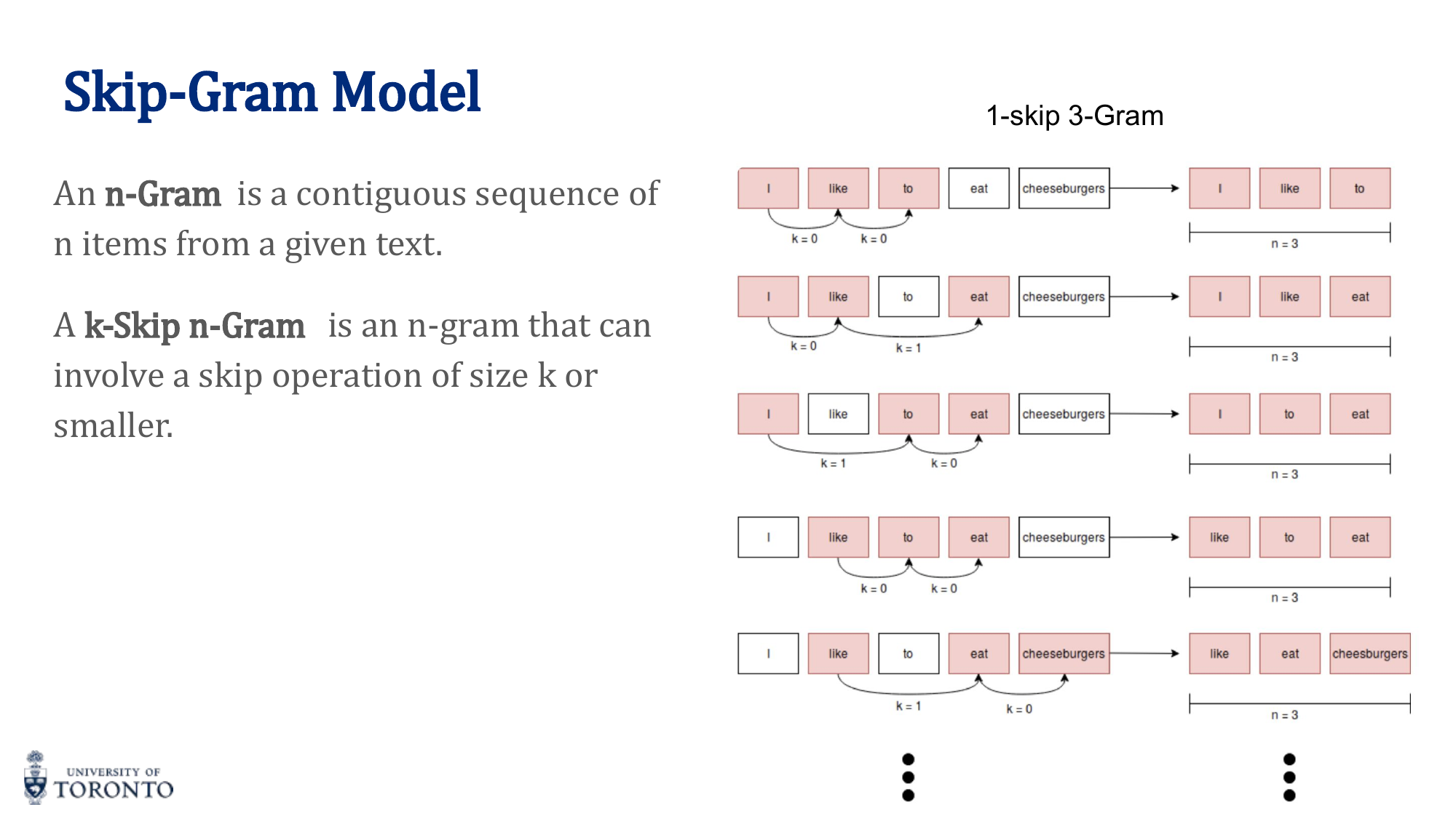
Skip-Gram vs. CBOW
- Skip-Gram: Predicts context words from a target word. Better for small datasets and rare words.
- CBOW (Continuous Bag of Words): Predicts the target word from context words. Faster and better for frequent words.
Solving Analogies with Word Embeddings
To solve “king - man + woman = ?”:
- Represent each word as a vector.
- Compute the target vector: vking - vman + vwoman
- Find the word whose embedding is closest to the target vector → “queen”
Limitation: Word embeddings do not capture word order or compositional meaning of sentences.
Image Captioning Model
To build a model that takes an image and describes it in natural language:
- Use a CNN to encode the image into a feature vector.
- Pass the image embedding as the input to an RNN at the <BOS> (beginning of sequence) token, instead of random initialization.
- Train end-to-end using auto-regressive (next token prediction) cross-entropy loss with teacher forcing.
- Data consists of pairs of (image, text).
Focus Area 9 • Guaranteed Marks • Do This First
Coding Cheat Sheet
Every Coding Question Follows These Patterns • 10 Marks
The Format — Expect It
The midterm coding question was 10 marks: (a) implement an nn.Module class [6] + (b) write a training loop [4]. The final will look the same. If you lock in the 7 patterns below, you lock in the coding marks.
Pattern 1 • The Training Loop
4 free marks. Identical for ANN, CNN, RNN, LSTM, GRU, Autoencoder. Never changes. Memorize.
# Inside the epoch/batch loop:
optimizer.zero_grad()              # 1. clear old gradients
outputs = model(inputs)            # 2. forward pass
loss = criterion(outputs, labels)  # 3. compute loss
loss.backward()                    # 4. backprop
optimizer.step()                   # 5. update weights
If You Forget Nothing Else
Write these 5 lines. That's 4/10 secured on any coding question.
The Full Training Function (epoch + batch loop)
The 5 lines above go inside two nested loops. This is the full template:
# ---- Setup (before training) ----
model     = MyModel()
criterion = nn.CrossEntropyLoss()
optimizer = torch.optim.Adam(model.parameters(), lr=0.001)
train_loader = DataLoader(dataset, batch_size=32, shuffle=True)

# ---- Epoch + batch loop ----
for epoch in range(num_epochs):
    total_loss = 0
    for inputs, labels in train_loader:
        optimizer.zero_grad()              # ┐
        outputs = model(inputs)            # │
        loss = criterion(outputs, labels)  # │ Pattern 1
        loss.backward()                    # │
        optimizer.step()                   # ┘
        total_loss += loss.item()
    print(f"Epoch {epoch+1}, Loss: {total_loss/len(train_loader):.4f}")
Two Loops, Always
Outer loop = epochs (one full pass through the entire dataset). Inner loop = batches (one gradient update per batch). The 5 Pattern 1 lines live inside the batch loop.
Common Exam Extras
loss.item()— converts tensor to Python float for logging; use this, notlossdirectly.model.train()before training,model.eval()before evaluating (toggles dropout / batch-norm behaviour).- Validation loop: same as training but wrap in
with torch.no_grad():and dropzero_grad/backward/step.
Pattern 2 • The nn.Module Skeleton
Every architecture fits this template. __init__ = what layers exist. forward = how data flows.
class MyModel(nn.Module):
    def __init__(self, ...):
        super(MyModel, self).__init__()
        # declare layers here

    def forward(self, x):
        # connect layers here
        return x
Pattern 3 • Which Loss Function?
| Task | Loss | Last Layer |
|---|---|---|
| Regression / Autoencoder | nn.MSELoss() |
Raw output (no activation) |
| Binary classification | nn.BCEWithLogitsLoss() |
NO sigmoid |
| Multi-class (most common) | nn.CrossEntropyLoss() |
NO softmax |
| GAN (D and G) | nn.BCEWithLogitsLoss() |
NO sigmoid |
The Rule That Burns Students
CrossEntropyLoss and BCEWithLogitsLoss apply softmax/sigmoid internally. Do NOT add them in your forward().
Pattern 4 • CNN
Formula: conv → relu → pool → conv → relu → pool → flatten → FC
# __init__
self.conv1 = nn.Conv2d(in_ch, out_ch, kernel_size)
self.pool  = nn.MaxPool2d(2, 2)
self.fc1   = nn.Linear(out_ch * H * W, num_classes)

# forward
x = self.pool(F.relu(self.conv1(x)))
x = x.view(-1, out_ch * H * W)   # flatten
x = self.fc1(x)
return x
Output Size Formula
out = (input - kernel + 2*padding) / stride + 1. Track dimensions layer by layer.
Pattern 5 • RNN / LSTM / GRU
Formula: embedding → rnn → take last hidden state → FC
# __init__
self.emb = nn.Embedding.from_pretrained(glove.vectors)
self.rnn = nn.LSTM(input_size, hidden_size, batch_first=True)
self.fc  = nn.Linear(hidden_size, num_classes)

# forward
x = self.emb(x)
h0 = torch.zeros(1, x.size(0), self.hidden_size)
c0 = torch.zeros(1, x.size(0), self.hidden_size)  # LSTM only!
out, _ = self.rnn(x, (h0, c0))   # LSTM: (h0, c0)  |  RNN/GRU: h0
return self.fc(out[:, -1, :])    # last hidden state
The ONE Difference
LSTM needs both h0 AND c0 passed as a tuple. Vanilla RNN and GRU only need h0. Everything else is the same.
Pattern 6 • GAN Training (the Label Trick)
# Train Discriminator: honest labels
real_labels = torch.zeros(batch_size)   # real = 0
fake_labels = torch.ones(batch_size)    # fake = 1
# concat real + fake, run through D, compute loss, D_optim.step()

# Train Generator: LYING labels
fake_images = G(noise)
outputs = D(fake_images)
labels = torch.zeros(batch_size)   # label fake as REAL to fool D
loss = criterion(outputs, labels)
loss.backward()
G_optim.step()
Remember
D and G have separate optimizers. Never mix them. Generator's trick is flipping the label.
Pattern 7 • Autoencoder
- Encoder: big → small (
Conv2d + MaxPool2dorLinear). - Decoder: small → big (
ConvTranspose2dorLinear). - Loss:
nn.MSELoss()between OUTPUT and INPUT (not labels!). - Denoising: add noise to input, reconstruct the clean version.
ConvTranspose2d Output Size
out = (input - 1) * stride - 2*padding + kernel_size
Common Gotchas — Quick Reference
super(ClassName, self).__init__()— always the first line in__init__.x.view(-1, N)— flatten for FC layers;-1infers batch size.BatchNorm2dfor conv,BatchNorm1dfor linear,LayerNormfor transformers/RNNs.nn.Dropout(p=0.3)— declare in__init__, use inforward; auto-disabled in eval mode.weight_decay=1e-8goes in the optimizer, not the model.- GloVe:
torchtext.vocab.GloVe(name='6B', dim=50). Distance:torch.norm(a - b). Similarity:torch.cosine_similarity(a.unsqueeze(0), b.unsqueeze(0)). - ResNet skip connection:
output = input + layer(input). - Transfer learning: load pretrained, freeze with
param.requires_grad = False, replace last FC layer.
5-Hour Cram Order
- Memorize Pattern 1 (training loop) cold — 4 marks locked.
- Practice Pattern 4 (CNN) and Pattern 5 (LSTM) once each on paper — they're the most likely.
- Learn Pattern 3 (loss table). Know which loss pairs with which last layer.
- Skim Patterns 6 and 7 if time remains.
Focus Area 10 • Every Exam • Shape & Param Questions
Dimensions & Parameter Counts
Output Sizing • Weight Shapes • Total Parameters
Why This Matters
Param-count and dimension-tracking questions appear on every exam. The 7 equations below cover every architecture you'll see.
1 • Output Dimensions (the 3 equations)
| Layer | Output Size Formula |
|---|---|
| Conv2d | \( H_{\text{out}} = \left\lfloor \dfrac{H - K + 2P}{S} \right\rfloor + 1 \) |
| MaxPool2d / AvgPool2d | \( H_{\text{out}} = \left\lfloor \dfrac{H - K}{S} \right\rfloor + 1 \) (P=0 typical) |
| ConvTranspose2d | \( H_{\text{out}} = (H - 1) \cdot S - 2P + K \) |
\( K \) = kernel size, \( P \) = padding, \( S \) = stride. Same formula for \( W_{\text{out}} \). Tensor shape: [B, out_channels, H_out, W_out].
Quick Check Defaults
If \( S=1,\ P=0 \): output shrinks by \( K-1 \). If \( S=1,\ P=\lfloor K/2 \rfloor \) ("same" padding): output size unchanged.
2 • Parameter Count per Layer
| Layer | # Parameters (with bias) |
|---|---|
| Conv2d\( (C_{\text{in}},\ C_{\text{out}},\ K) \) | \( (K \cdot K \cdot C_{\text{in}} + 1) \cdot C_{\text{out}} \) |
| Linear\( (D_{\text{in}},\ D_{\text{out}}) \) | \( (D_{\text{in}} + 1) \cdot D_{\text{out}} \) |
| Embedding\( (V, D) \) | \( V \cdot D \) (no bias) |
| BatchNorm2d\( (C) \) | \( 2C \) (\( \gamma,\ \beta \) per channel) |
| LayerNorm\( (D) \) | \( 2D \) |
| RNN\( (D, H) \) | \( H \cdot (D + H + 1) \) |
| GRU\( (D, H) \) | \( 3 \cdot H \cdot (D + H + 1) \) (3 gates) |
| LSTM\( (D, H) \) | \( 4 \cdot H \cdot (D + H + 1) \) (4 gates) |
| Pool / ReLU / Dropout / Flatten | \( 0 \) (no learnable params) |
Drop the "+1" for bias=False
If the question says "no bias": drop the + 1. Conv2d becomes \( K \cdot K \cdot C_{\text{in}} \cdot C_{\text{out}} \). Linear becomes \( D_{\text{in}} \cdot D_{\text{out}} \).
3 • Weight Matrix Shapes (for dimension questions)
Vanilla RNN — input \( x_t \in \mathbb{R}^{D} \), hidden \( h_t \in \mathbb{R}^{H} \):
LSTM — one set per gate (\( f, i, c, o \) = 4 sets total):
GCN layer — \( N \) nodes, \( F \) input features, \( F' \) output features:
Transformer attention — \( d_{\text{model}} \) = model dim, \( h \) = heads, \( d_k = d_{\text{model}} / h \):
4 • Shape Tracking Through a CNN
Write the shape after every layer. This is how you avoid the flatten bug on exam day.
# Input image: 3 channels, 32x32
x: [B, 3, 32, 32]

# Conv2d(3, 16, kernel=3, padding=1)  → same-size
x: [B, 16, 32, 32]

# MaxPool2d(2, 2)                    → halve H/W
x: [B, 16, 16, 16]

# Conv2d(16, 32, kernel=3, padding=1)
x: [B, 32, 16, 16]

# MaxPool2d(2, 2)
x: [B, 32, 8, 8]

# Flatten  →  32 * 8 * 8 = 2048
x: [B, 2048]

# Linear(2048, 10)
x: [B, 10]
The Flatten Rule
The first FC layer's input size is Cout × Hout × Wout from the last conv/pool output. Forget this and your model breaks with a shape mismatch.
5 • RNN / LSTM Input & Output Shapes
| Tensor | Shape (with batch_first=True) |
|---|---|
Input x |
[B, T, D] |
Initial hidden h0 (and c0 for LSTM) |
[num_layers, B, H] |
Output out (all timesteps) |
[B, T, H] |
Last hidden state out[:, -1, :] |
[B, H] → feed to FC |
B = batch, T = sequence length, D = input/embedding dim, H = hidden size.
6 • Worked Example: Count Total Parameters
Simple CNN: Conv2d(3, 16, 3) → pool → Conv2d(16, 32, 3) → pool → Linear(32·6·6, 10)
7 • Worked Example: LSTM Parameters
nn.LSTM(input_size=100, hidden_size=128):
Same setup with GRU → multiply by 3 instead of 4 = \( 87{,}936 \). Vanilla RNN → multiply by 1 = \( 29{,}312 \).
Exam-Day Checklist
- Write the shape after every layer — don't skip steps.
- For param counts: (weights) + (biases), always check if bias is present.
- Conv2d: \( K \cdot K \cdot C_{\text{in}} \cdot C_{\text{out}} + C_{\text{out}} \). Linear: \( D_{\text{in}} \cdot D_{\text{out}} + D_{\text{out}} \).
- LSTM = \( 4\times \), GRU = \( 3\times \), RNN = \( 1\times \) the \( H(D+H+1) \) template.
- Pool / ReLU / Dropout / Flatten → 0 parameters. Don't count them.
Practice Examination
Final Exam Review
20 Questions • ~100 Points Total
Question 1 • 3 Points
Define the vanishing gradient problem. Which activation functions are most susceptible to it, and how does ReLU address it?
Question 2 • 3 Points
What is the difference between a hyperparameter and a parameter in neural network training? Give two examples of each.
Question 3 • 4 Points
Explain why random search is generally preferred over grid search for hyperparameter optimization.
Question 4 • 5 Points
A convolutional layer receives an input of size 32 × 32 × 3 and applies 16 filters of size 5 × 5 with stride 1 and padding 2. (a) What is the output size? (b) How many trainable parameters does this layer have (including biases)?
Question 5 • 3 Points
What is the purpose of pooling layers in a CNN? Name two common types.
Question 6 • 6 Points
Compare and contrast AlexNet, VGGNet, and ResNet. For each, state (a) the key architectural innovation, and (b) why it was significant.
Question 7 • 5 Points
Explain the difference between feature extraction and fine-tuning in transfer learning. When would you choose one over the other?
Question 8 • 5 Points
Explain how a Variational Autoencoder (VAE) differs from a standard autoencoder. What is the reparameterization trick and why is it necessary?
Question 9 • 3 Points
What is the difference between Skip-Gram and CBOW in word2vec? Which is better for rare words and why?
Question 10 • 3 Points
Why is cosine similarity preferred over Euclidean distance for comparing word embeddings?
Question 11 • 6 Points
Draw or describe the LSTM cell architecture. Name all three gates and explain the role of each. How does the cell state address the vanishing gradient problem?
Question 12 • 4 Points
What is mode collapse in GAN training? Why does it happen and what strategies can mitigate it?
Question 13 • 7 Points
Explain the Scaled Dot-Product Self-Attention mechanism step by step. What are Q, K, and V? Why is the scaling factor √d_k used? Write the full formula.
Question 14 • 5 Points
What is Multi-Head Attention? Why is it better than single-head attention? Write the formula.
Question 15 • 5 Points
Compare BERT and GPT. How do they differ in architecture, pre-training objective, and use cases?
Question 16 • 4 Points
Why do Transformers need positional encoding? What happens if you remove it? Describe the sinusoidal encoding scheme.
Question 17 • 5 Points
Explain the message-passing framework in GNNs. What three operations does each layer perform? Why must the aggregation function be order-invariant?
Question 18 • 6 Points
Compare GCN and GAT. What problem does the naive GCN (H = ReLU(AXW)) have, and how is it fixed? How does GAT improve upon GCN?
Question 19 • 8 Points
You are building a system to classify molecules as toxic or non-toxic. Each molecule is represented as a graph where atoms are nodes and bonds are edges. (a) What type of GNN task is this? (b) Describe the full pipeline from input graph to classification output. (c) What aggregation function would you use and why? (d) How would you handle the fact that different molecules have different numbers of atoms?
Question 20 • 8 Points
You need to build a model to generate realistic face images conditioned on attributes (e.g., "male, smiling, brown hair"). (a) Compare using a VAE vs a conditional GAN for this task — list advantages and disadvantages of each. (b) Describe the architecture and training procedure for the conditional GAN approach. (c) What is one common failure mode and how would you detect it?
Study Progress
Exam Checklist
Track your preparation • Progress saved locally
Week 2 — ANNs Part I
Week 3 — ANNs Part II
Week 4 — CNNs Part I
Week 5 — CNNs Part II
Week 6 — Unsupervised Learning
Week 7 — Word Embeddings
Week 8 — RNNs
Week 9 — GANs
Week 10 — Transformers
Week 11 — GNNs